Modern weather and climate prediction models, such as the one used in ECMWF’s Integrated Forecasting System (IFS), are complex multi-component software systems simulating Earth system processes. At the heart of each Earth system model lies its dynamical core. Its purpose is to solve the equations that govern atmospheric motions. Those equations link all atmospheric dynamical and physical processes which provide ‘source terms’, in other words the ‘fuel’ that generates all types of atmospheric motions. Here we present a new, efficient and simple iterative algorithm to compute semi-Lagrangian advection, which deals with the transport of heat, momentum, moisture and atmospheric constituents. It will be introduced in the next upgrade of the IFS planned for 2023.
Advection in the IFS
Although the equations of motion of the dynamical core are continuous, only discrete forms can be solved on a computer. The solution starts from a set of initial conditions, the so-called analysis, and evolves step by step until the final forecast time. Sophisticated numerical methods must be used, which stem from rigorous mathematical analysis, to ensure accurate and stable calculations. At the same time, considerable effort is spent to engineer such methods to work fast on modern supercomputing architectures.
A crucial part of each dynamical core is the advection scheme. This is the part of the model time-stepping scheme which calculates the transport of heat, momentum, moisture and atmospheric constitutes around the globe, given the winds at each point in time. The ECMWF dynamical core uses a semi-Lagrangian (SL) advection scheme, which ensures that an accurate solution, with very little numerical dispersion, can be produced stably with long time steps. The latter means that it is computationally efficient, as we can use fewer steps to produce a given forecast. It is also multi-tracer efficient, which means that, when transporting many atmospheric species (gas tracers), its overhead is small compared with other methods.
The SL scheme is combined with a semi-implicit scheme, ensuring that all dynamical core equations are solved stably and accurately using long time steps. The introduction of the SL technique in the IFS in 1991 was a major enhancement of its capability to deliver efficiently successive resolution upgrades and improvements. This is an old scheme, but because of its success in global atmospheric modelling, it has been continuously developed, enhanced, and improved to match ever-evolving and challenging modelling and computer hardware requirements. What is currently used is an evolution of the original scheme, enhanced to allow accurate and computationally efficient predictions for modern high-resolution requirements and to support atmospheric composition modelling.
With increasing resolution and model complexity and the introduction of reduced precision to speed up the forecast model, we found that components of the advection scheme had become slow and that they required special treatment to preserve the required accuracy. For this reason, part of the advection scheme has been rewritten, using a mathematical formulation that leads to a faster but equally accurate solution.
The semi-Lagrangian advection scheme
Atmospheric motions and energy exchanges alter the transported fields (moisture, air density, temperature, momentum etc.). Any change incurred is the outcome of different adiabatic and diabatic processes (pressure differences, rotation, diffusion, heating, evaporation/condensation, friction etc.), which are calculated separately during each model time step. However, advection is a passive process which moves atmospheric substances (fields) without altering their nature at all. SL advection achieves combining effectively the Lagrangian method with the fixed grid required by the physics. To do this, it uses the concept of backward trajectories: for each model grid point, it must trace backwards in space and time the origin of the Lagrangian trajectories formed by air parcels as they are advected (passively transported) by the wind. Calculation of backward trajectories implies that, at each time step, each parcel will arrive at a grid point, which is also called ‘arrival point’. The origin of each trajectory, called the ‘departure point’, in general lies between grid points. It is computed solving the so-called trajectory differential equation dr/dt=V(r,t), where r denotes the coordinates of an air parcel and V(r,t) the wind field acting on it, which is variable in space and time.
Hence, when restricted to advection, the time evolution of a transported variable on each grid point is determined by two steps in a SL method: the first step is to find the Lagrangian departure points, and the second is to estimate the value of the transported variable at these locations. The latter is done by interpolating neighbouring grid point values. Having good accuracy in both computational steps is essential for an accurate forecast. Inaccurate departure point calculations in the vertical will generate large temperature errors and negatively impact the flow, while inaccurate horizontal point calculations will introduce phase errors in Rossby waves and forecast the wrong location of cyclones. Inaccurate interpolation will generate substantial amplitude errors in all weather features and will poorly forecast the intensity of weather phenomena.
In this article, we will concentrate on the departure point calculations. These are computed by solving a discretised version of the trajectory equation. This discretised equation is ‘implicit’ in nature (the unknown departure point appears in the left- and the right-hand side of the equation). It can be solved with a mathematical technique called ‘fixed point iteration’. This is an iterative method which produces approximations to the solution. The number of iterations needed for the algorithm to converge to the solution varies considerably in different regions of the atmosphere. In areas where the wind flow is nearly uniform with weak gradients, it converges rapidly. Here, one or two iterations are enough. However, near the jet stream or tropical cyclones, where the horizontal and vertical wind shear is large, convergence is slow, and more iterations are needed. The time step length affects the rate of convergence. The quantity that determines this rate is the Lipschitz number, which is the product of time step and the norm of the wind shear.
The iterative scheme used in the IFS is called SETTLS (Stable Extrapolation Two-Time-Level Scheme). Although this looks like a simple algorithm when the equations are expressed on a Cartesian framework, its simplicity is lost when spherical polar coordinates are used. For example, curvature effects need to be accounted for, and to obtain the latitude and the longitude of each departure point, the inversion of a 3x3 nonlinear system of equations is required. This adds computational expense and complexity in the code such that the final scheme seems to bear little resemblance to the original SETTLS. Furthermore, when the departure point calculations are carried out in reduced precision (‘single-precision’ rather than ‘double-precision’ was introduced recently in the IFS to speed up execution), near the poles the accuracy is reduced. It was therefore necessary to keep big parts of this calculation at high precision.
A new algorithm for departure points
Over the last few years, external funding from the EU-funded ESCAPE project helped scientists at ECMWF, in collaboration with external partners from several Member States and the EU, to study in detail the computational performance of fundamental algorithms of the IFS dynamical core as well as physical parametrizations, such as the cloud scheme. Several self-contained software modules were produced, the so-called dwarfs. One of these dwarfs focused on semi-Lagrangian advection. The same method, based on SETTLS, was replicated in the dwarf, but it was implemented differently. Modern data structure and object-oriented programming concepts that were available in ECMWF’s Atlas library were used. In practice, this meant that it was easier to implement and test different algorithms for semi-Lagrangian advection.
Among the alternatives explored were iterative algorithms for the departure points, which were computing the semi-Lagrangian trajectories using an equivalent geocentric Cartesian framework, mitigating singularity problems associated with spherical polar coordinates in the polar regions. At the same time, alternative non-iterative algorithms were explored that were cheaper in terms of computation and communication. However, testing suggested that the iterative approach was essential for accuracy. Therefore, a Cartesian iterative algorithm based on SETTLS, which was also simpler, was ported into the operational IFS code environment to be explored further in detail.
At the same time, there were parallel efforts at ECMWF. The plan was to remove the polar singularity existing in spherical coordinates and to improve tangent-linear and adjoint integrations used in the data assimilation system. This was to be done by re‑designing parts of the departure point calculations to work with Cartesian coordinates. Such ideas matured after discussions with an ECMWF Member and Co-operating State scientist (Jan Mašek, Czech Hydrometeorological Institute). An option was added in the IFS to compute the departure points with parts of these calculations in a Cartesian coordinate framework. More specifically, the wind vectors were transformed into Cartesian coordinates before they were interpolated at the departure point estimates at each iteration of the SETTLS scheme. This amended algorithm, which was fully blended with the existing scheme, still had parts computed directly in spherical polar coordinates. It was making the overall calculation slightly more complex and expensive. However, it motivated further developments and fusion with the ideas that were discussed in the previous paragraphs.
Having the earlier experience from the Atlas-based preliminary implementations and experiments, it was clear that a further big step could be taken to simplify and reduce the cost of the computations of SETTLS by rewriting the entire algorithm in Cartesian coordinates. An additional advantage was that the resulting iterative scheme was ‘rotation matrix-free’, unlike the algorithm which it replaced. The latter requires that the wind vectors, after being interpolated at the departure point during iterations, are multiplied by a rotation matrix to account for the change in orientation of the local coordinate system that describes them due to the Earth’s curvature. Furthermore, the calculation of latitude–longitude of the departure points was greatly simplified, no longer needing the inversion of nonlinear system of equations. The improved arithmetic scaling due to measuring distances from the centre of the Earth also meant that there was no need to approximate any terms or to keep any parts of the relevant code in double precision in single-precision runs. Finally, the original departure point calculation code was squeezed to less than 50%, and the associated tangent-linear and adjoint versions of the nonlinear model became much simpler. These are greatly beneficial features from the efficiency and maintenance point of view.
Accelerating the departure point calculation
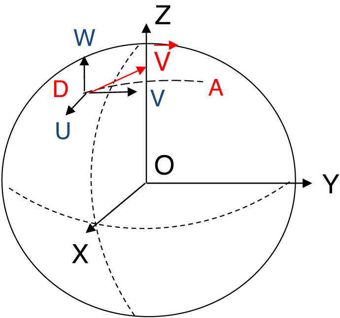
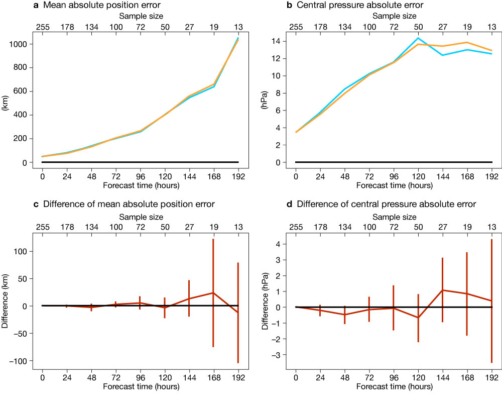
The Cartesian coordinate algorithm for computing the departure points described so far is much more concise than its predecessor. Nevertheless, it is not faster than the default scheme of the IFS. The reason is that, within a Cartesian geocentric system (see Figure 1), movement on a 2‑dimensional spherical surface takes place in 3-dimensional (X, Y, Z) space and requires three wind components to be described (U, V, W). These can be obtained from the wind components (u, v) in spherical coordinates by a simple transformation (see Table 1). On balance, given that the new Cartesian algorithm was simpler, despite needing an extra dimension its cost was similar compared with the original scheme. Could we accelerate these calculations further? Indeed, it turned out to be possible, but before explaining how this was done, we need to highlight some further aspects of these calculations and their dependency with the model time step.
We mentioned earlier that the quantity that determines how many SETTLS iterations are needed to compute the departure points is the Lipschitz number, i.e. the product of time step and the norm of the wind shear. At each resolution upgrade, the model time step is carefully selected to give the highest possible forecast accuracy consuming the least possible high-performance computing resources in the fixed time-critical window of ECMWF operations. For accuracy reasons, the ratio of the time step to grid-spacing must remain roughly the same as the model resolution increases. However, testing that took place before the upgrade to 9 km horizontal resolution in high-resolution forecasts (HRES) in March 2016 showed undesirable side effects: unphysical stratospheric flow structures were seen over tropical cyclones, as well as large areas of increased upper-air field errors in the winter season above big mountain ranges. The origin of such skill degradations was found in the departure point calculation and the fact that, with successive model improvements, for efficiency reasons, we had pushed the time step to values that resulted in higher Lipschitz numbers. With long time steps, more iterations were needed, and thus iterations were increased from three to five. This increased the cost of the advection scheme but reduced the overall model cost as it allowed a 12.5% longer time step.
Although increasing the number of iterations to five resulted in a net gain in efficiency, the departure point calculation became an expensive part of the model, roughly taking up 7% of total CPU time. There were attempts to reduce this cost, for example by combining SETTLS in the vertical with a very economical scheme for computing the longitude and latitude of the departure points, invented by John McGregor (Commonwealth Scientific and Industrial Research Organisation, Australia). In the end, the most practical and economical idea was born in a coffee break with a member of ECMWF’s Scientific Advisory Committee, Prof. Eigil Kaas, in 2019. After reviewing options, his suggestion was to test initialising the departure point iterations using the previous time step departure points rather than using the explicit Euler predictor to produce these. Indeed, after some special treatment for the vertical part of the calculation was added, this idea worked very well and was adopted (for details, see Diamantakis & Váňa, 2022).
Verifying the new algorithm
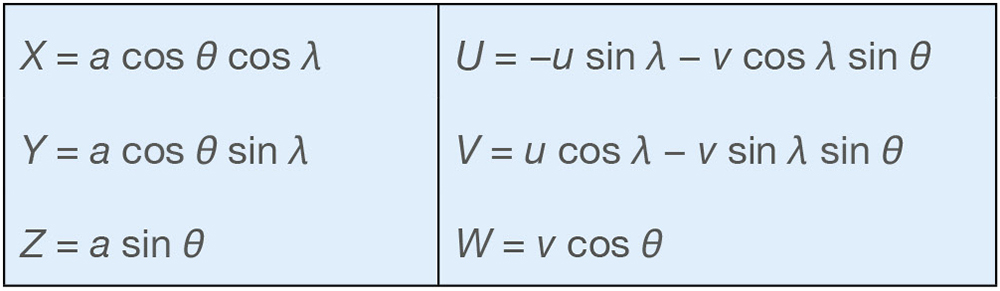
The good accuracy of this new, faster algorithm can be demonstrated with a simple forecast experiment. Figure 2 shows a plot of the 500 hPa geopotential height root-mean-square error (RMSE) difference of 30 forecasts with the old SETTLS implementation in polar spherical coordinates with three iterations from the old operational SETTLS with 5 iterations (left) and of the new SETTLS implementation in Cartesian coordinates with three iterations from the old SETTLS with 5 iterations (right). We notice that a significant increase in RMSE appears over the Himalayas when the number of iterations is reduced in the old scheme, which is completely absent in the new scheme: it can achieve the same accuracy with a 40% reduction in the number of iterations, saving approximately 2–3% of total CPU model time.
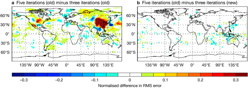
There was further detailed testing of this new development in the IFS over different seasons, cycles, forecast tests and resolutions, ranging from standard 10‑day forecasts to long climate type runs and from 130 km to 2.5 km resolution. All verification tests confirmed that reducing the number of iterations in the new scheme has no impact on accuracy, with a hint of a slight improvement in cases of strong cross-polar flow. An interesting comparison is shown in Figure 3, where the mean absolute position error and the minimum pressure error (core pressure) are compared for two different sets of consecutive forecasts of the Atlantic 2020 hurricane season, verified against Best Track observations. The first set (cyan line) is produced by standard IFS forecasts in double precision using the old SETTLS scheme, which uses polar spherical coordinates and five iterations. The second set (orange line) is produced by an IFS version which uses the new Cartesian coordinate SETTLS with three iterations, with all model computations in single precision. The result demonstrates the overall quality of the entire single-precision development and the new development: with significantly less computation, the same accuracy is achieved.
Conclusion and further work
In this article, we discussed an alternative formulation for a crucial part of the IFS advection scheme, the algorithm that computes the departure point of the semi-Lagrangian trajectories. This alternative implementation, which will be introduced in IFS Cycle 48r1, brings some important benefits. It needs fewer iterations to find the solution, hence it requires less computation, but it is equally accurate. It is a simpler algorithm that is better suited for reduced-precision calculations as well as for calculations near the poles.
This new development could widen the possibilities for future improvements. For example, it could aid efforts to revise and optimise the parallel communication strategy for the semi-Lagrangian advection scheme. This could be done by implementing alternative ‘thin halo’ communication on-demand approaches, which will reduce the memory and communication cost in future high-resolution, massively parallel weather forecast simulations. Furthermore, it could facilitate work to develop a stochastic departure point framework. The aim is to capture flow-dependent uncertainty from the dynamics in regions where it is known that the numerical algorithms can produce larger errors due to the complexity of the flow. The simplicity of the new scheme offers an advantage in implementing such approaches.
Further reading
Diamantakis, M. & F. Váňa, 2022: A fast converging and concise algorithm for computing the departure points in semi-Lagrangian weather and climate models. Q. J. R. Meteorol. Soc., 148, 670–684.
Diamantakis, M. & L. Magnusson, 2016: Sensitivity of the ECMWF model to semi-Lagrangian departure point iterations. Mon. Wea. Rev., 144, 3233–3250.
M. Hortal, 2002: The development and testing of a new two-time-level semi-Lagrangian scheme (SETTLS) in the ECMWF forecast model. Q. J. R. Meteorol. Soc., 128, 1671–1687.