On 23 March 2022, the Copernicus Climate Data Store (CDS) and Atmosphere Data Store (ADS) were successfully migrated from Reading (UK) to ECMWF’s new data centre in Bologna (Italy). The CDS and ADS are part of the EU-funded Copernicus Climate Change Service (C3S) and Copernicus Atmosphere Monitoring Service (CAMS) run by ECMWF. They are deployed on a private, on-premises cloud infrastructure, running OpenStack. The service is composed of over 250 virtual machines, running on 30 physical servers, each having 48 CPUs and around 190 gigabytes of memory. This article describes how genetic algorithms are used to find an optimal placement of virtual machines onto physical hosts in order to optimise the service offered by the CDS/ADS. This is an example of the increasing use of machine learning at the Centre, in this case to optimise the performance of a service.
Function of virtual machines
Some of the virtual machines serve the CDS/ADS catalogue and its search engine, others manage the queue of incoming user requests and broker them to the right data source or compute service. Virtual machines also process the requests and handle the download of results back to users. In addition, tens of virtual machines host a disk-only MARS (Meteorological Archival and Retrieval System) server, serving two petabytes of selected ERA5 climate reanalysis data and CAMS data. All these services communicate with each other over a virtual network, and they may be CPU, I/O or network intensive, depending on their purpose.
Every virtual machine has some memory allocated to it, as well as a number of virtual CPUs, virtual disks and virtual network interfaces. OpenStack will not run more virtual machines on the same physical host than the number that fits in the physical memory available. On the other hand, it will allow for more virtual CPUs to be allocated on the same host than the number of available physical CPUs (by a factor of two). This enables a better use of resources as many virtual machines are mostly idle, waiting for work to do. But when some of the services are very busy, virtual machines that share the same host will ‘steal’ CPU resources from each other.
A
Genetic algorithms
Genetic algorithms (GAs) simulate evolution to find the best solution to a problem. Solutions are represented by a vector of symbols, usually bits, floating-point numbers, integer numbers or characters. The vectors are referred to as ‘chromosomes’ and their elements are referred to as ‘genes’.
The algorithm starts by generating a large number of random solutions (known as the ‘population’). For each solution (also called ‘individuals’), a ‘fitness’ is computed; the higher the fitness, the closer it is to the best solution to the problem. A new population is then created by selecting the fittest individuals (‘parents’); new individuals are created by ‘mating’ the parents, i.e. by creating new solutions whose genes are a combination of the genes of the parents, in a process called ‘cross-over’. Finally, a few genes of each individual are randomly changed, in a process called ‘mutation’; this allows solutions to be considered that were not in the population. The process is then repeated for several ‘generations’. The fittest individual of the last iteration is considered to be the best solution.
Even though GAs explore the space of solutions randomly, they often provide useful results, given a large enough population and a large number of generations, as well as carefully selected cross-over and mutation strategies. GAs are a useful tool when estimating the fitness of a solution is easy to implement. For more details on genetic algorithms, see: en.wikipedia.org/wiki/Genetic_algorithm.
It should also be noted that, when a virtual machine reads from or writes to a virtual disk, this results in network transfers between the compute hosts and the storage hosts that compose an OpenStack installation. This means that all networking and I/O performed by the virtual machines of a physical host will make use of the network interfaces of that host. On the other hand, network transfers between the two collocated virtual machines will be very fast, as the data remains within the same host and no actual networking is taking place.
As a result, to ensure a performant system, virtual machines that are running services that consume a lot of CPUs and I/O should be kept apart, while those that transfer large amounts of data between themselves should be collocated on the same physical hosts.
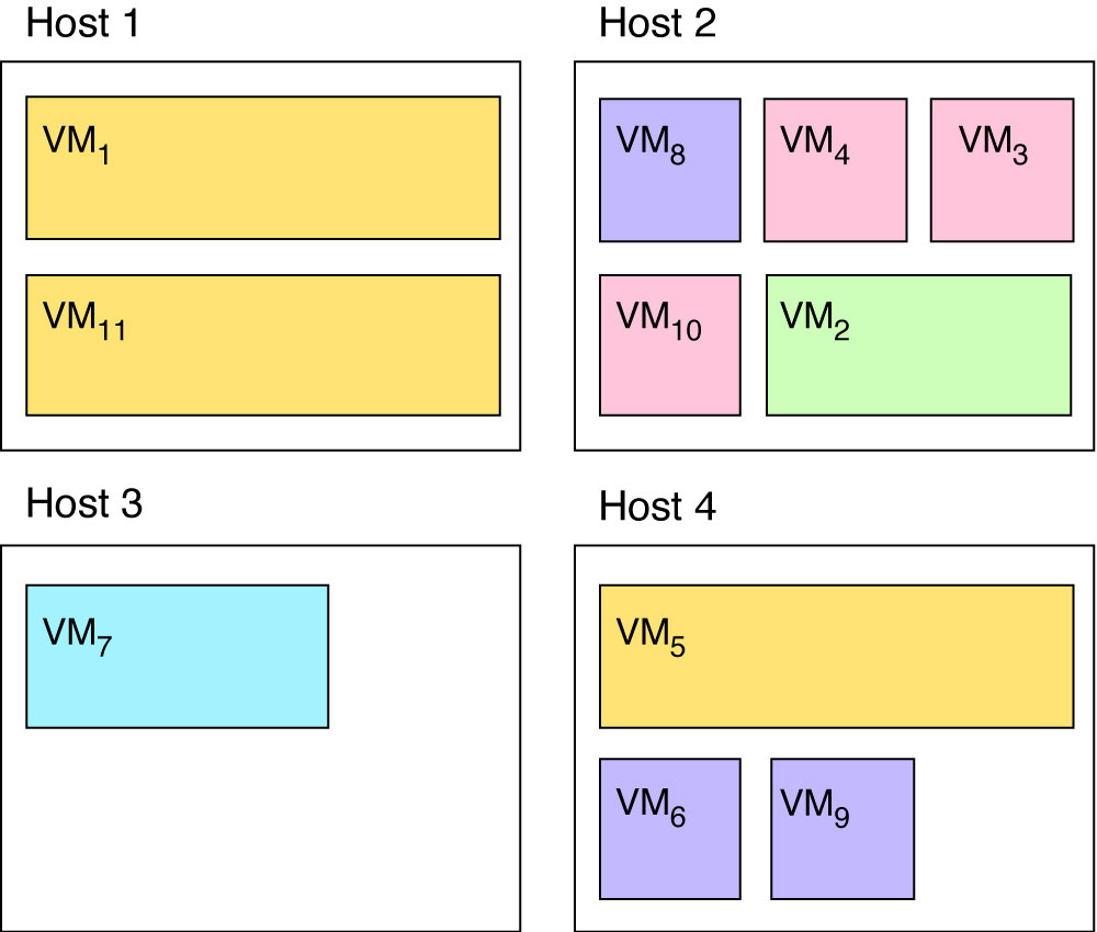
Figure 1 illustrates a situation where virtual machines are placed on physical hosts more or less randomly. Given the following constraints:
- virtual machines of the same colours should not be placed on the same host
- purple and pink virtual machines must be collocated pairwise
- resource usage must be evenly distributed amongst hosts,
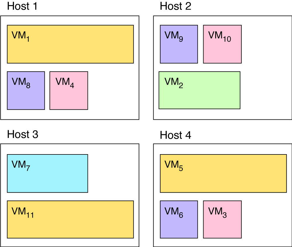
a genetic algorithm should output a solution such as the one given in Figure 2.
Implementation
OpenStack provides a command-line tool to query the state of the system and perform actions on it. With that tool, it is possible to build a map of the system, finding out which virtual machines run on which physical hosts, how much memory and CPU they use, etc. Furthermore, the tool also allows an administrator to migrate a virtual machine from one physical host to another, without interrupting the service.
Chromosome encoding
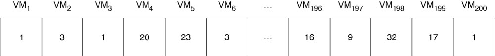
The tool is first used to establish a list of physical hosts as well as characteristics such as the number of CPUs and available memory. Then the current distribution of virtual machines and their resource requirements is mapped, also in terms of CPUs and memory. The resulting information is encoded in a ‘chromosome’ as follows: the physical hosts are numbered from 1 to Nhosts; similarly, the virtual machines are numbered from 1 to Nvm; we use a vector to represent a possible placement of virtual machines onto hosts: the vector has Nvm elements, one per virtual machine, each representing on which physical host the corresponding virtual machine is located (Figure 3).
Using that encoding, the placement in Figure 1 would be [1,2,2,2,4,4,3,2,4,2,1] and the placement in Figure 2 would be [1,2,4,1,4,4,3,1,2,2,3].
Affinity
We define the ‘affinity’ between two virtual machines as the fact of whether they should be located on the same hardware or on different hosts. This information is based on the virtual machine names and is provided in a configuration file.
Fitness function
To compute the fitness of a possible placement, we consider which of the following ‘hard constraints’ are violated:
- the sum of the memory requirement of all virtual machines sharing the same host must not exceed the amount of physical memory of that host
- two virtual machines that should not be collocated must not be on the same host
- two virtual machines that should be collocated must not be on different hosts.
We also consider the following ‘soft constraints’:
- the standard deviation of the number of allocated virtual CPUs on all hosts must be minimal (this ensures that the CPU load is evenly spread within OpenStack)
- the number of virtual machines to be relocated is minimal (although this is not very important).
The fitness of the solution is then defined as:
fitness(s) = – (hard_constraints × large_weight + soft_constraints)
Initial population and setup
We find that generating the initial population by including the current placement of virtual machines within the system and its permutations will help the genetic algorithm to converge faster than starting from a purely random population.
The default setup for the genetic algorithm is to run for 100 generations over a population of 1,000 individuals and to use the ‘steady-state’ selection method, a ‘single-point crossover’ strategy, and a random mutation of genes.
Software
The software described in this article is written in Python and relies on the OpenStack command-line tool to interact with the infrastructure. It uses the PyGAD Python library for building the genetic algorithms. The software can be found at https://github.com/ecmwf-lab/vm-placement.
Results
Given 30 hosts and 250 virtual machines, the algorithm runs for under a minute on a modern laptop and outputs the list of virtual machines that need to be migrated to different physical hosts. The OpenStack command-line tool is then used to perform the live migration.
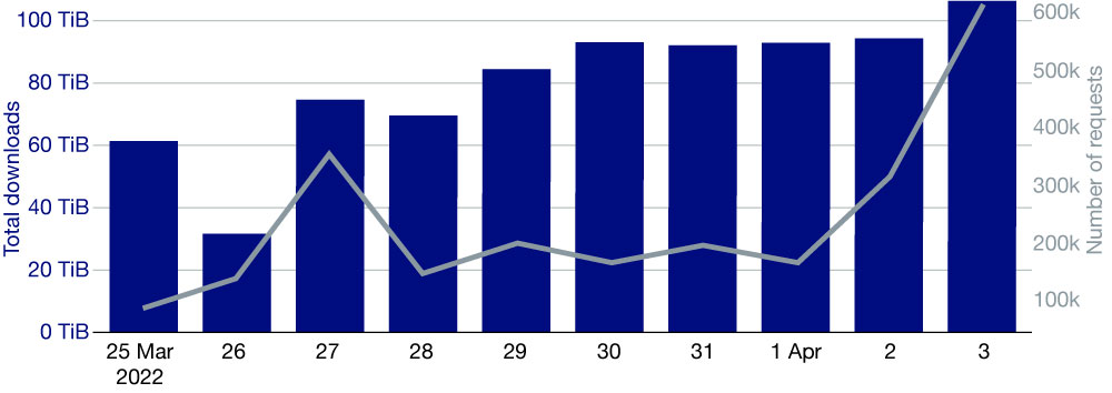
The CDS/ADS is a complex system, and its performance depends on many factors, some of which are due to the load generated by the users’ activity. It is therefore difficult to measure which part of any improvement is due to using an optimal placement of the virtual machines. Nevertheless, a few days after tuning the CDS, we reached a record: over 106 TiB delivered in 24 hours, in 600,000 user requests (Figure 4).
A multi-year project to modernise the CDS/ADS started in February this year. The CDS/ADS will continue to be hosted in OpenStack and in addition will make use of Kubernetes, which will improve our control of virtualisation. The software will be enhanced to make use of that finer control.