
Air pollution is a global public health risk. The World Health Organization (WHO) estimates that 4.2 million people worldwide, including hundreds of thousands of people in Europe, die prematurely each year because of poor ambient air quality and that 91% of the world’s population live in areas where air quality fails to meet WHO guidelines. It is therefore important to provide air quality forecasts on global, regional and local scales to support public health authorities and policy-makers and to enable vulnerable people to take preventative action during pollution episodes. The Copernicus Atmosphere Monitoring Service (CAMS), implemented by ECMWF on behalf of the European Union, provides services related to atmospheric pollution on the global and European scale, combining information from models and observations to enable a continuous assessment of the air we breathe. For its global forecasting system, CAMS uses a wide range of atmospheric composition observations from satellites to improve the initial conditions for its daily 5-day forecasts. The latest satellite to provide such data for CAMS is Sentinel-5 Precursor (S5P). S5P was launched by the European Space Agency (ESA) in October 2017 and is the first satellite mission in Europe’s Copernicus Earth observation programme to be dedicated to monitoring atmospheric composition. Tests carried out at ECMWF show that the use of S5P data on ozone and carbon monoxide improves the CAMS analysis of atmospheric composition, which is produced using ECMWF’s Integrated Forecasting System (IFS). S5P ozone data are now assimilated operationally by CAMS, and the assimilation of other S5P species is expected to follow later in 2019.
Trace gases observed by S5P/TROPOMI
S5P carries the Dutch-developed TROPOspheric Monitoring Instrument (TROPOMI), which provides high-resolution measurements in the ultraviolet (UV), visible (VIS), near infrared (NIR) and shortwave-infrared (SWIR) part of the spectrum. This wide spectral range enables several atmospheric trace gases to be retrieved, e.g. ozone (O3), nitrogen dioxide (NO2), sulphur dioxide (SO2) and formaldehyde (HCHO) from the UV-VIS, and carbon monoxide (CO) and methane (CH4) from the SWIR part of the spectrum. These species are all included in the CAMS system, making TROPOMI the perfect instrument to provide observations for CAMS at the unprecedented horizontal resolution of about 3.5 km x 7 km for the UV-VIS and 7 km x 7 km for the SWIR products. See Box A for details on the species that are relevant to monitoring and forecasting air quality.
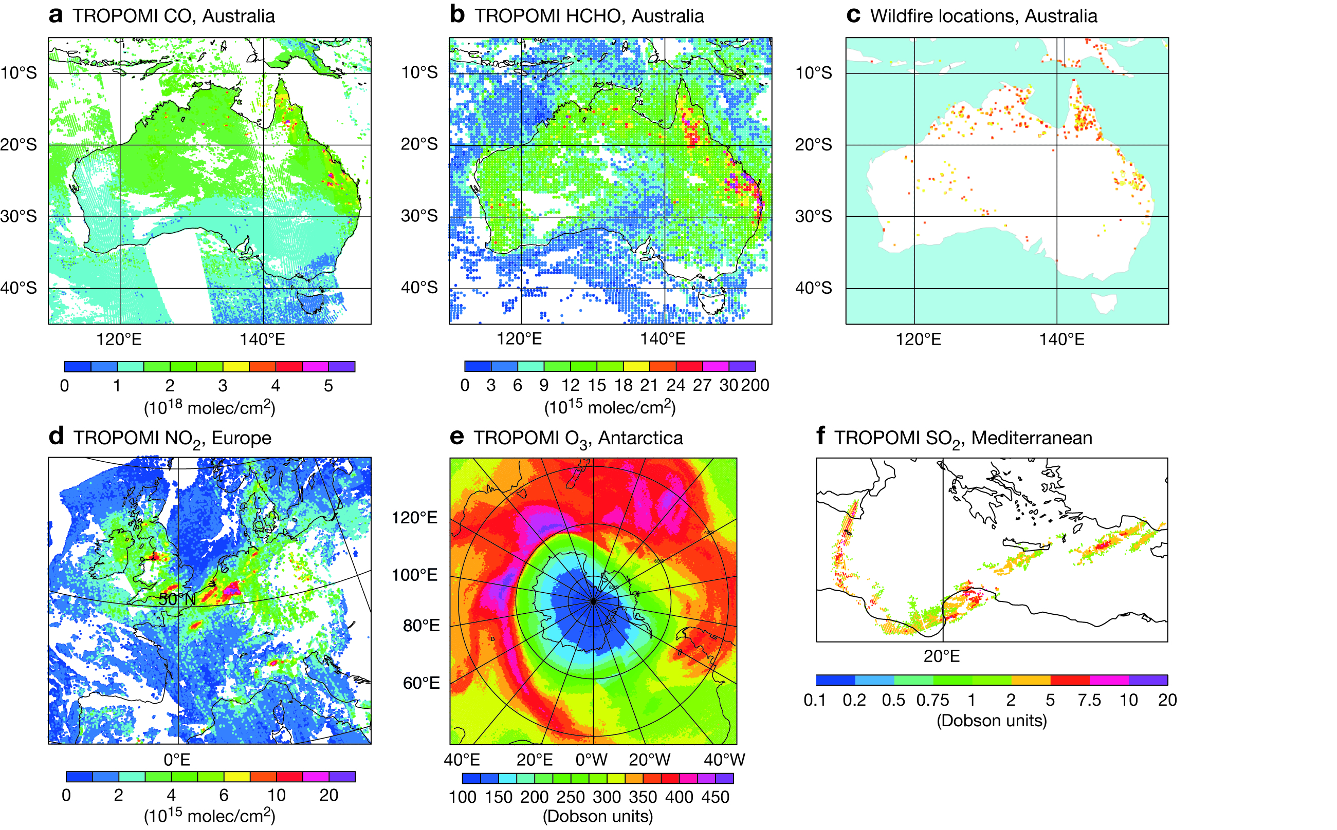
Figure 1 shows examples of TROPOMI data products. It shows elevated CO and HCHO columns over Australia on 2 December 2018 in areas strongly affected by bushfires at the time. A map of NO2 values over Europe on 27 June 2018 illustrates that TROPOMI’s resolution is good enough to detect plumes of pollution coming from individual cities (e.g. London, Paris, Hamburg). The map also shows high NO2 values in the Netherlands, the Ruhr region in Germany and the Po valley in northern Italy as well as high NO2 values from the Saddleworth Moor fires in northeast England. Figure 1e shows low total column O3 values in the southern hemisphere ozone hole area on 1 October 2018, and Figure 1f shows elevated values of volcanic SO2 over the eastern Mediterranean from the eruption of the Mount Etna volcano in Sicily on 26 December 2018.
Monitoring and assimilating S5P O3 data
During the first nine months after launch, the S5P satellite was in its so-called commissioning phase, which mainly served for functional testing, in-flight calibration and testing of processing chains. Nevertheless, ECMWF and ESA agreed to start monitoring these early data in the IFS. The model fields are interpolated in time and space to the location of the observations, and model equivalents of the observations are calculated (i.e. what TROPOMI would see if the state of the atmosphere corresponded to the interpolated model fields). This enables us to calculate temporal and spatial statistics of the differences between the observations and collocated model fields and gives us information on how the data compare to the daily CAMS analyses, which are constrained by various other satellite instruments. At the monitoring stage, the data are not actively used in the assimilation and therefore do not influence the analysis and subsequent forecast. Once the quality of the data has been established, active assimilation of the new data is tested in research experiments and the impact of their assimilation on the CAMS analysis is assessed with the help of independent validation data.
A
Some species relevant to air quality
For the purposes of air quality monitoring and forecasting, it is essential to have access to observational data on levels of ozone, nitrogen dioxide, carbon monoxide, formaldehyde and sulphur dioxide in the atmosphere.
Ozone: While stratospheric ozone is important and protects us from some of the sun’s harmful UV radiation, tropospheric ozone at high concentrations can be harmful to humans, animals and vegetation. Tropospheric ozone is formed when nitrogen oxides (denoted NOx, which means NO2 and NO), CO, and volatile organic compounds react in the presence of sunlight. In urban areas in the northern hemisphere, high ozone levels in the lower troposphere usually occur during spring and summer. Over the Antarctic, stratospheric ozone destruction during austral spring leads to strong and rapid depletion of the ozone layer, the so‑called ‘ozone hole’.
Nitrogen dioxide: NO2 is another key atmospheric pollutant, which is produced by road traffic, power plants and fossil fuel or biomass burning processes. Higher up in the troposphere, lightning and aviation also produce NOx. NO2 has a short lifetime so that concentrations are larger over land than in the cleaner air over the oceans. The largest concentrations are found over industrial and urban regions of the eastern US, California, Europe, China and Japan.
Carbon monoxide: CO has natural and anthropogenic sources. It is emitted from soils, plants and the ocean, but its main sources are incomplete fossil fuel and biomass burning. It is also produced by oxidation of CH4 and other hydrocarbons. The highest CO concentrations are found over the industrial regions of Europe, Asia and North America. CO has a lifetime of several weeks and can serve as a tracer for regional and inter-continental transport of polluted air. The main loss process is the reaction with the hydroxyl radical.
Formaldehyde: HCHO is produced by the oxidation of methane and volatile organic compounds and also by incomplete combustions of hydrocarbons. It has sources from industrial processes, wildfires and biogenic emissions from vegetation. HCHO has a short lifetime of a few hours, making it a good indicator of hydrocarbon emission areas.
Sulphur dioxide: SO2 also has natural and anthropogenic sources. It is emitted from volcanoes and produced by coal-fired power stations, industrial processes or other fossil fuel burning activities (e.g. cars or ships). The lifetime of SO2 in the troposphere is a few days, in the stratosphere it can be several weeks. Volcanic eruptions that put ash and SO2 high into the atmosphere can be a major risk to aviation.
TROPOMI total column O3 (TCO3) retrievals going back to 26 November 2017 were monitored with the CAMS system in this way. Time series of TROPOMI TCO3 observations and differences between the observations and the CAMS analysis (analysis departures) are shown in Figure 2a,b in the form of Hovmöller diagrams, which show TCO3 observations and departures by latitude and time of year, averaged over the respective latitude circle. The highest O3 columns are found in the northern hemisphere spring and the lowest values over Antarctica during the ozone hole season. Even at this early stage, the TROPOMI TCO3 data generally agreed well with the CAMS analysis over large parts of the globe. They also agreed well with TCO3 retrievals from the Ozone Monitoring Instrument (OMI) and the Global Ozone Monitoring Experiment-2 (GOME-2), which are routinely assimilated by CAMS (not shown). However, the TCO3 near-real-time data from TROPOMI showed some retrieval anomalies at high latitudes and over snow/ice (e.g. Antarctica), where the differences with the CAMS analysis and the other datasets are larger (Figure 2c). These differences come mainly from the surface albedo climatology that is used in the near-real-time TROPOMI TCO3 retrieval. This climatology has a coarser horizontal resolution than the TROPOMI TCO3 data, which leads to problems in areas where there are large changes in reflectivity from pixel to pixel, e.g. pixels that are/are not covered by snow/ice. More details about this can be found in Inness et al. (2019a).

The impact of assimilating TROPOMI TCO3 observations was tested in research experiments, again going back to November 2017. Assimilating the observations was found to have a small positive impact on the ozone analysis compared to TCO3 data from ground-based spectrometers (not shown) and ozonesonde observations in the tropical troposphere (Figure 3a) as well as in the troposphere and parts of the stratosphere over Antarctica (Figure 3b) during September to October 2018. There was also an improved fit to In-service Aircraft for a Global Observing System (IAGOS) data at West African airports (Figure 3c). In other areas, the impact was small. The overall impact of the TROPOMI data is relatively small because the CAMS analysis is already well constrained by several other ozone retrievals that are routinely assimilated (GOME-2, OMI, MLS, SBUV/2 and OMPS). Averaged over the periods February–April and September–October 2018, the differences between experiments with and without assimilation of TROPOMI data are within 2% for TCO3 and within 3% in the vertical for seasonal mean zonal mean O3 mixing ratios, with the largest relative differences found in the troposphere. It should be noted that the current CAMS system cannot fully exploit the high resolution of the TROPOMI data at present because its horizontal grid spacing of 40 km is coarser than that of the TROPOMI data.

Because of the small positive impact on the CAMS analysis, it was deemed to be beneficial to include the data actively in the operational CAMS system. The assimilation of the near-real-time TROPOMI TCO3 data in the operational CAMS system was started in December 2018. Beyond the immediate impact, the addition of TROPOMI data makes the CAMS system significantly more resilient in case some of the older instruments whose retrievals are currently assimilated by CAMS stop working.
Monitoring and assimilating TROPOMI CO data
The use of TROPOMI total column CO (TCCO) data has been explored by CAMS in research experiments. CAMS routinely assimilates thermal infrared (TIR) TCCO retrievals from the Measurement of Pollution in the Troposphere (MOPITT) instrument and the Atmospheric Sounding Interferometer (IASI). TROPOMI data successfully capture the global TCCO distribution (Figure 4a) with relatively high TCCO values in the northern hemisphere, lower values in the southern hemisphere, and high TCCO values over the biomass burning areas in the tropics and the areas of high anthropogenic pollution over India and southeast Asia. However, there are some systematic differences between the TROPOMI data and the CAMS TCCO analysis (Figure 4b and 4c), particularly in the northern hemisphere at low solar elevations north of 40°N, where TROPOMI has higher TCCO values than CAMS. Since the CAMS system is known to underestimate CO in the northern hemisphere extratropics, particularly during winter/spring and in the lower troposphere, some of these differences are likely to be the result of a CAMS model bias.

When TROPOMI data are assimilated in the CAMS system, they lead to increased CO values in the extratropics and lower values in the tropics, with TCCO changes of up to 30% at high northern latitudes (Figure 5a). Even though the TROPOMI data are total columns, their assimilation has a large impact on the vertical structure of the CAMS CO analysis because of different sensitivities of the TROPOMI SWIR and the MOPITT and IASI TIR retrievals to CO in the atmosphere. While the TIR retrievals are most sensitive to CO in the mid-troposphere, TROPOMI SWIR measurements are sensitive to the integrated amount of CO along the light path, including the contribution of the planetary boundary layer (the atmospheric layer that interacts with the surface). The largest absolute and relative changes due to the TROPOMI TCCO assimilation are found in the lower and upper troposphere (Figure 5b), i.e. the part of the atmosphere that is not well constrained by the assimilated MOPITT and IASI TIR retrievals.

The assimilation of TROPOMI TCCO leads to an improved fit to European Global Atmosphere Watch (GAW) surface CO observations over Europe (not shown) and IAGOS aircraft CO profiles in several areas (Figure 6). Particularly noteworthy is that it reduces the long standing low bias of the CAMS system over Europe. Relative to IAGOS, there are also reduced biases over Australasia, Southeast Asia and in parts of the free troposphere over India and West African airports. However, in some areas the fit to IAGOS observations is degraded, and the assimilation leads to increased negative biases over India and West Africa in the lower and upper troposphere. There is also an overestimation of surface CO relative to GAW observations at Cape Verde and a degraded fit to CO data from the Total Carbon Column Observing Network (TCCON) in the northern hemisphere, while the bias at the Lauder TCCON site in the southern hemisphere is reduced (not shown; see Inness et al., 2019b). More work is required, including work on the bias correction of the TROPOMI TCCO data, before the data can be assimilated in the operational CAMS system.

Use of S5P in the operational CAMS system
Near-real-time O3 and NO2 from TROPOMI were included in monitoring mode in the operational CAMS system in July 2018. This was followed by CO in November 2018 and HCHO and SO2 in December 2018. CH4 retrievals are not available in near-real time but will be monitored in the CAMS greenhouse gas analysis, which runs a few days behind real time. CAMS started to assimilate TROPOMI TCO3 data in its daily operational air quality forecasts on 4 December 2018 and assimilation tests with near-real-time NO2, CO and volcanic SO2 from TROPOMI are under way. It is hoped that the assimilation of all these species will be activated in the operational CAMS system during 2019.
Further reading
Inness, A., J. Flemming, K.-P. Heue, C. Lerot, D. Loyola, R. Ribas, P. Valks, M. van Roozendael, J. Xu & W. Zimmer, 2019a: Monitoring and assimilation tests with TROPOMI data in the CAMS system. near-real time total column ozone, Atmos. Chem. Phys. Discuss., 19, 3939–3962, doi:10.5194/acp-19-3939–2019.
Inness, A., I. Aben, A. Agusti-Panareda, T. Borsdorff, J. Flemming, J. Landgraf & R. Ribas, 2019b: Monitoring and assimilation tests of TROPOMI total column carbon monoxide data in the CAMS system. ECMWF Technical Memorandum No. 838.