
For 30 years, ECMWF’s Metview software has been providing straightforward ways to access, process and visualise ECMWF forecasts and related data. Many workflows involve the exploration of large datasets. This can include data inspection, filtering and plotting. This type of work has traditionally been performed using Metview’s Graphical User Interface (GUI), but in recent years new environments such as Jupyter notebooks have become popular, especially for teaching in virtual environments. This article describes new features in Metview’s Python interface designed to meet these needs.
Working with multiple GRIB files
Grid-based and spectral output fields from numerical weather prediction (NWP) models, such as ECMWF’s Integrated Forecasting System (IFS), are produced in binary GRIB format. When a GRIB file is read into Metview using the Python programming language, the data object returned is called a Fieldset. Metview has always had features for combining multiple GRIB files into a single Fieldset, but recent developments have made it even easier. The Fieldset constructor can now take a list of paths to GRIB files, or even a wildcard. The following example shows two ways of loading multiple GRIB files into a Fieldset:
import metview as mv

my_gribs = ["/path/data_a.grib", "/path/ data_b.grib"]

fs1 = mv.Fieldset(path=my_gribs)

fs2 = mv.Fieldset(path="/path/*.grib")
The features described in the rest of this article apply to all Fieldsets, whether obtained from single or multiple GRIB files. They also apply to datasets, described later.
Exploring the contents of GRIB data
It is not immediately obvious exactly what data lie in a collection of GRIB files. Metview’s GUI provides a tool to quickly examine the contents of a GRIB file. In a non-GUI Python environment, such as Jupyter notebooks, new functions provide these capabilities.
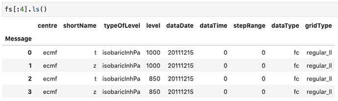
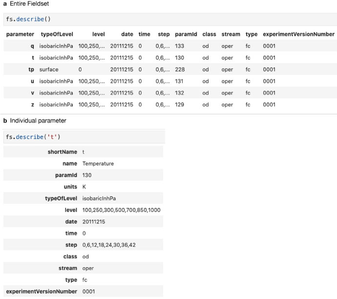
The most straightforward one is the ls() function. This prints details of each and every field in a Fieldset, with customisable columns (see Figure 1). For larger datasets, the describe() function groups the GRIB messages by parameter and gives a summary for quick inspection. It can also be used to delve deeper into an individual parameter (see Figure 2). In both functions, the output is customised to take advantage of the formatting capabilities available in a notebook environment.
Plot widget for Jupyter
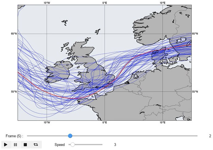
When using Metview’s GUI, data are plotted by default into an interactive plotting widget called the Display Window, which provides many features to navigate through the different fields. In a Jupyter environment, a new plotting widget was developed to allow the user to easily navigate the fields. Plot frame selection is available via the slider control, and continuous playback and looping are also possible (see Figure 3). For the purpose of integrating the plots into a saved version of the notebook, the widget can be deactivated.
New plotting functions
Metview offers a rich plotting interface with fully customisable graphical end products. However, setting up plots like the ones showcased in the Metview Gallery requires several steps, including data management, layout generation and most importantly styling, resulting in lengthy code for some plots. This approach is fully acceptable when a new product is being developed, but in a training environment or when we just want to explore the data, it can be a big overhead. To overcome this difficulty, a high-level plotting interface was added to Metview’s Python interface. It comprises a set of functions, each capable of generating a certain type of plot in a single line of code using predefined settings. These include plot_maps(), plot_diff_maps(), plot_xs(), plot_stamp(), plot_rmse(), plot_cdf(). All these functions take their default style settings from the newly developed style library, which includes predefined map areas, map styles and data visualisation styles (contouring, wind, symbol and storm track plotting) allowing for specialisation per plot type. For map-based plots, the contouring uses the ecCharts style when it is available for the given parameter. However, like all the other style settings, it can be overridden by the user.
Figure 4 shows how plot_diff_maps() can be used to generate a fixed-layout plot showing the difference between a potential vorticity forecast and the analysis using default settings.

Selecting fields
Some training environments, such as OpenIFS user workshops, require the handling of many thousands of GRIB fields. In these cases, Metview’s traditional GRIB filter using the read() function can struggle to select subsets of fields in acceptable time, especially if run multiple times over the same data. To handle these large cases, a new Python-based GRIB filtering function called select() was written. It uses pandas DataFrames to internally index the GRIB fields, and the cost of running it multiple times over the same data is virtually the same as the cost of running it once. An additional difference to the read() filter is that any ecCodes keys can be used in the filter query, making it usable with a wider variety of data than that which comes from the MARS archive.
Another new feature is a convenient shorthand notation for selecting fields from a Fieldset. The Python indexing operator can be used to select fields based on parameter, level and level type. The following pairs of lines are equivalent:
z = fs.select(shortName="z")

wind = fs.select(shortName=["u", "v"], level=500)
and
z = fs["z"]

wind = fs["wind500"]
Datasets
Metview has been extensively used in OpenIFS training courses to help participants carry out case studies and evaluate their simulations. Gaining from this experience and building on the new Python components discussed in this article, the dataset concept was introduced to Metview. A dataset is a collection of data files packaged together with a tailored style library, which, combined with a set of Python scripts or notebooks, can form a curated environment for a training course. The GRIB data in a dataset is always pre-indexed, offering optimised access to the fields. We can use describe() to inspect the contents and select() to extract data from it. When a dataset is loaded, its style library automatically becomes the current one and high-level plot functions like plot_maps() will automatically pick up the settings from it, guaranteeing that the plots look right by default and do not require further customisation. Datasets are not distributed with Metview but can be regarded as external resources that can be freely created, distributed and shared.
Use in new NWP training course
In 2021, ECMWF offered a new training course: A Hands-on Introduction to NWP Modelling (Keeley et al., 2021). The practical modelling exercises were to a large part based on a case study featuring a storm event which took place in 2016. The participants were given the task to apply changes to some of the model’s physics parametrizations and to investigate how this would affect the simulated development of the storm and its associated local weather impacts.
In group work, the participants were encouraged to use their own forecasting knowledge to select appropriate meteorological parameters to assess the storm development as modelled by OpenIFS. Correspondingly, a wide range of model fields and diagnostics needed to be written out by the model to offer the opportunity to look at different aspects. Given the time constraints during the training course, it was necessary to be able to process and visualise all parameters and diagnostics in a quick and efficient way and allow for comparison between different forecast experiments. Also, due to the virtual delivery of the course within a Jupyter notebook environment, and having limited resources for each training lab instance on the European Weather Cloud, the visualisation needed to be Python-based, easy to use and quick with low computational requirements, and it had to produce inline figures in the Notebooks.
The new Python-based Metview functions were used by each course participant to combine the output from their own reference forecast and sensitivity experiments into a Metview dataset object. Additional GRIB Fieldsets from the operational analyses, for the same forecast time period and interpolated to the same grid resolution, were added to the participant’s OpenIFS model results to allow comparison. When additional forecast experiments were carried out later, they could also easily be added to the existing dataset.
The plotting functions developed for the dataset came with reasonable default presets. Without any prior experience with Metview, a wide variety of plots of instantaneous and accumulated model fields could be quickly created with different styles (regional mask, map projections, selected time steps for animation). Participants who wished to experiment with the style presets had the option to modify the default settings by editing a small number of configuration files. Difference plots between experiments highlighted changes in the model’s representation of the storm caused by altered model physics. The time slider allowed the animation of the storm evolution within the Jupyter notebook inline figures.
Future
With greater availability of ECMWF data through an open data policy, it is more important than ever to have straightforward facilities to inspect, filter, process and visualise data within a standard workflow. Raw model output data, which can be of greater volume and spatial complexity, should also fit into the same workflow. By evolving developments such as those described above, we will continue to support the Python community to make the best use of all our data.
Availability
Metview is installed on ECMWF’s computing platforms, including the Member and Co-operating State server ecgate. For use external to ECMWF’s computing platforms, Metview is also available as a binary installation on the conda platform, available through the conda-forge channel with one of these commands:
conda install metview -c conda-forge

conda install metview-batch -c conda-forge # no GUI installed
The Python interface can be installed with either of these commands:
conda install metview-python -c condaforge

pip install metview
Metview’s Python documentation has been moved to readthedocs and can be accessed here: https://metview.readthedocs.io/en/latest/. Jupyter notebooks illustrating the concepts described in this article can also be found there.
Further reading
Keeley, S., X. Abellan, G. Carver, M. Köhler, S. Kertész & I. Russell, 2021: Making training mobile, ECMWF Newsletter No. 168, pp. 12–13.