The middle of February 2022 was very cyclonic over north-western Europe, with three named storms affecting this area in one week. Cyclone Eunice (also known as Nora and Zeynep) was one of these; it delivered major wind-related impacts in many countries. Here we focus on Eunice and in particular on the gust predictions for the British Isles for 18 February.
Eunice’s life cycle
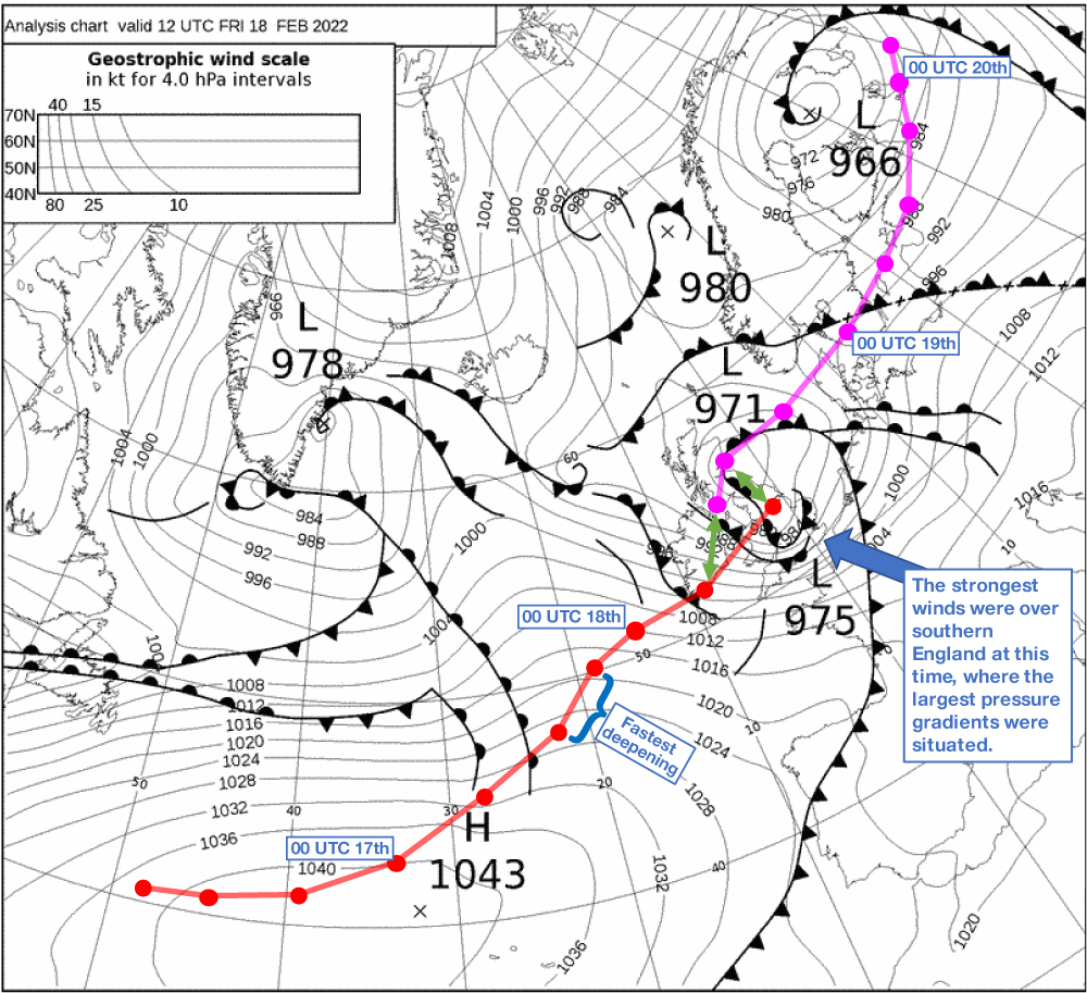
The life cycle of Eunice is represented by coloured tracks on the synoptic chart figure. Eunice started out early on 16 February, in diminutive wave form, on a complex cold front situated west of the Azores. The cyclone then intensified as it translated rapidly east-northeastwards, being driven along in the developmental right-entrance region of an upper level jet. Wind speeds at 300 hPa peaked at around 85–90 m/s, which is strong but not exceptional. As the system crossed the jet core on 17 February, explosive development ensued. The most rapid deepening phase – which for Eunice was approximately 12–18 UTC on 17 February – tends to be just before the risk period for a ‘sting jet’ in a cyclone’s life cycle. This is critical because sting jets tend to lead to exceptional surface wind speeds over land and sea. Indeed, on the evening of 17 February, image sequences of Eunice showed some hallmarks of a sting jet over the Atlantic, notably evaporating cloud head tips, although these only lasted a few hours. The fact that rapid deepening occurred well away from land helped spare the land-based population from the worst of Eunice’s winds. Nonetheless, winds associated with the ’cold jet’ phase, which follows any sting jet phase and tends to last much longer, did deliver major impacts across northern Europe. In the cold jet phase, one mechanism that fuels downward momentum transfer, to deliver very strong surface gusts, is destabilisation via daytime insolation. Such a process seems to have enhanced gust strength over the south of the UK on 18 February, and over Poland and the Baltic States on 19 February.
Over the Atlantic, Eunice’s life cycle mirrored the classic evolution of an explosively developing cyclone. Over the British Isles, however, there was a departure from this, as the storm split into two centres: the former low (red track on the synoptic chart figure) eventually decayed as a newly developed centre to the north (magenta track) took over. This second centre then continued on an east-northeastward trajectory across northern Europe, eventually decaying about four days after Eunice’s genesis.
Wind gust forecasts
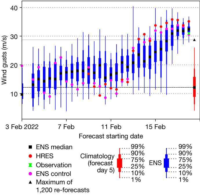
The forecast evolution figure shows how maximum wind gust forecasts over London Heathrow Airport on 18 February evolved from 3 February. The distribution from the ensemble re‑forecast-based model climate valid for forecast day five is shown as the red box-and-whisker symbol, with the maximum in the sample of 1,200 model climate forecast fields highlighted as a triangle. The maximum observed wind gust at the airport was 31 m/s, according to SYNOP reports. More than a week before the event, the ensemble system predicted a risk for windier-than-normal conditions. The forecast from 12 February already had high Extreme Forecast Index (EFI) values over northern Europe six days ahead. While the signal gradually started to increase in the ensemble for extreme gusts over Heathrow in the next few days, both the high-resolution forecast (HRES) and the ensemble (ENS) control forecast saw a jump towards an extreme level on 13 February. They stayed on the higher end (above the 75th percentile) of the ensemble distribution for the next three days. The lower level of risk implied by the ensemble at this stage is notable for this case, but it is impossible to judge the ensemble performance from one specific case. It could have been that this storm was more predictable than appreciated by the ensemble at that stage, favouring the unperturbed members. Ongoing research at ECMWF is investigating whether the ensemble has too much spread during cyclonic conditions.
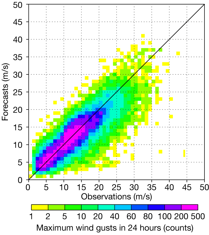
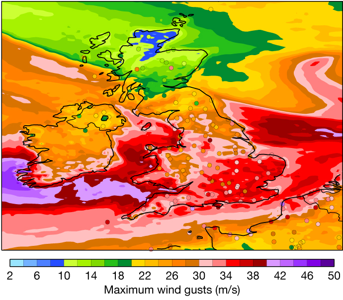
Storm Eunice brought very strong wind gusts of more than 30 m/s quite widely over southern England on 18 February. As can be seen in the plot on predicted and observed maximum wind gusts, the HRES also produced gusts of very high magnitude over the affected areas, but even close to the event HRES gusts were generally a few m/s stronger than observation reports. We will therefore have a closer look at the statistics of the wind gusts during the stormy period (12–20 February). In the Integrated Forecasting System (IFS), wind gusts are computed by accounting for turbulent and convective gustiness using a formula which includes an empirical parameter, Cugn, and a tuning convective mixing parameter, Cconv. To address the increasing positive forecast biases in recent years, the computation of wind gusts has been tuned in the current operational cycle of the IFS by reducing Cugn from 7.71 to 7.2 and Cconv from 0.6 to 0.3. This change has resulted in reduced forecast biases for wind gusts. As illustrated in the scatter plot image, there is good correspondence between forecast and observations over Europe during the stormy period in February. The gust factor (ratio between gusts and mean wind) also improved – there is a better match between the forecast and observations.
Contrasting errors
Whilst the gust forecast bias is generally small, in individual cases errors of different sign may occur. For example, the overprediction that we saw for Eunice contrasts with an underprediction for storm Franklin, which arrived a few days later, on 21 February. It could well be that different wind-gust phenomena (e.g. sting jet, cold jet, meso-scale convection systems) have different biases, although we must also acknowledge that the accuracy of the synoptic pattern forecast will play a major role for the prediction of wind gusts, with complex evolutions, such as the low-splitting observed for Eunice, being especially challenging.