
On 11 June 2019, ECMWF implemented a substantial upgrade of its Integrated Forecasting System (IFS). IFS Cycle 46r1 includes changes in the model and in the data assimilation procedure used to generate the initial conditions for forecasts. The upgrade has had a very positive impact on the skill of medium-range and extended-range ensemble forecasts (ENS) and medium-range high-resolution deterministic forecasts (HRES). It follows the implementation of IFS Cycle 45r1 in June 2018, which brought coupling to all ECMWF forecasts, from one day to one year ahead, by including ocean and sea-ice models in the HRES configuration.
Cycle 46r1 is the culmination of the work of many across ECMWF and brings major changes in many areas, including:
- In data assimilation: continuous data assimilation (an extra 4D-Var outer loop, an increase from 6 to 8 hours in the early-delivery assimilation window length, and an extension in the observation cut-off time); twice the number of members in the Ensemble of Data Assimilations (EDA); weakly-coupled data assimilation for sea-surface temperature in the tropics; consistent spatial interpolation of the model to observation locations in trajectories and minimisations; use of the EDA to calculate Jacobians in the soil-moisture analysis.
- In the use of observations: assimilation of the SMOS neural-network soil-moisture product; assimilation of SSMIS-F17 satellite data at 150h GHz and GMI satellite data at 166 GHz; improved use of land/sea mask in the field of view for microwave imagers; introduction of inter-channel observation error correlations for ATMS and geostationary water-vapour channels; slant path calculations for geostationary radiances; usage of geostationary radiances at higher zenith angles; consistent infrared aerosol detection.
- In the model: improvements in the convection scheme (entrainment, CAPE closure, shallow convection); activation of long-wave scattering in the radiation scheme; 3D rather than 2D aerosol climatology; correct scaling of dry mass flux in the diffusion scheme; improvement of the tangent linear and adjoint of the semi-Lagrangian departure point scheme in the polar-cap area; new parametrization for wind input and open ocean dissipation of the wave model; increase in the frequency of the ensemble radiation time step from 3 hours to 1 hour.
Data assimilation and observations
The continuous data assimilation scheme enables the use of later-arriving observations and, crucially, decouples the starting time of the assimilation calculations from the observational cut-off time. This permits the beneficial introduction of an additional outer loop without affecting delivery time. In addition, the early-delivery assimilation window length has been increased from 6 hours to 8 hours, thus ensuring that all observations that have arrived can be assimilated. For more details, see Lean et al. (2019).
The number of EDA members has increased from 25 to 50. The computational resources required are roughly the same as before as a result of efficiency improvements. The increase in the number of EDA members improves the HRES analysis by providing better background error variance and covariance estimates. Furthermore, it is now possible to assign a unique EDA perturbation to each ensemble forecast member, which makes the ensemble forecast members exchangeable. For more details, see Lang et al. (2019).
In the newly developed ocean–atmosphere weakly-coupled data assimilation, the atmospheric analysis sea-surface temperature in the tropics is taken from the ECMWF OCEAN5 near-real-time analysis, rather than from the OSTIA product directly. This results in improved forecast scores for near-surface temperature and humidity in the tropics compared to the analysis. For more details, see the article on weakly coupled data assimilation in this Newsletter.
For the surface analysis of soil moisture, the Simplified Extended Kalman Filter (SEKF) described by de Rosnay et al. (2013) has been significantly upgraded to improve computational efficiency, by computing its Jacobians directly from the EDA rather than with perturbed nonlinear trajectories. This reduces the SEKF computing cost, compared to previous IFS cycles, by more than a factor of three in the operational HRES configuration. The EDA-Jacobian approach in the SEKF also enhances the coupling between the land and atmospheric assimilation systems by ensuring more dynamic Jacobian estimates than in the previous finite-difference approach.
Cycle 46r1 has introduced a package of changes to microwave all-sky assimilation. This includes the assimilation of SSMIS‑F17 satellite data at 150h GHz and GMI satellite data (vertical and horizontal polarisation radiances) at 166 GHz, which bring new information on humidity and wind over tropical and subtropical oceans, as well as improving the use of the land–sea mask in the field of view for microwave imagers. Each microwave observation has a footprint depending on its frequency. We use the 10 GHz footprint for AMSR2 and GMI and the 19 GHz footprint for SSMIS-FOV to compute how the land–sea mask is affected by this footprint. This land–sea mask is more accurate than that used in Cycle 45r1, which depends on the resolution of each loop.
Inter-channel observation error correlations have been introduced for ATMS satellite data, which results in ATMS observations being assimilated, on average, with more weight. This has resulted in significant and consistent improvements in the fit of the short-range forecasts used in the data assimilation system (first-guess fit) to independent observations sensitive to temperature, humidity and wind, indicating improved forecasts of these variables.
Similarly, inter-channel observation error correlations have been introduced for geostationary satellite water vapour channels, affecting SEVIRI (Meteosat Second Generation) and AHI (Himawari) instruments, to provide the best first-guess fit to water vapour channels on other instruments, as well as impact at longer lead times.
A further upgrade to the use of geostationary radiances is to account for slanted paths within the radiative tansfer calculation. This change enables us to use data up to zenith angles of 74°, thus improving coverage at the edges of the geostationary disks. This is particularly significant in the North Atlantic, where previously a significant amount of Meteosat‑10 data was not used.
In addition, the SMOS (Soil Moisture and Ocean Salinity) neural-network soil moisture satellite product is now assimilated along with the ASCAT level‑2 surface soil moisture satellite product. The impact of using SMOS neural network data and the EDA Jacobians on medium-range weather forecasts is near neutral. However, there is a small but significant improvement in 2‑metre temperature forecasts in the short range in the northern hemisphere.
Main modelling improvements
In Cycle 46r1, the ENS radiation time step has been reduced from 3 hours to 1 hour, as is already the case for the HRES. Forecast skill is improved almost everywhere as a result, including a substantial error reduction for 2‑metre temperature forecasts. Much of the improvement can be attributed to the faster coupling of radiation, clouds and the surface. Over tropical land areas, the root-mean-square error in low clouds has been reduced by as much as 15%. More frequent radiation updates incur an overall cost increase in the operational ENS of only about 3%. This was made possible in part because the new radiation scheme introduced in IFS Cycle 43r3 (ecRad) is significantly cheaper than its predecessor.
In addition, long-wave radiation scattering has been turned on in the radiation scheme, which leads to a slight warming of the surface and a reduction in the root-mean-square error in tropospheric temperature forecasts of around 0.5%. A key innovation in the implementation is to represent longwave scattering by clouds but to neglect it for aerosols (Hogan & Bozzo, 2018). This brings virtually all the benefits whilst enabling several optimisations to be performed, such that the overall cost of the radiation scheme when longwave scattering is included is very slightly reduced.
The 2D aerosol climatology used in the radiation scheme has been replaced by a new 3D aerosol climatology. This change has some positive impacts on lower tropospheric temperature and winds, especially along coastlines affected by seasonal biomass burning interacting with boundary layer clouds. Bigger positive impacts can be seen in the stratosphere, where the root-mean-square error of the temperature field in the 50–100 hPa layer near the summer pole decreases by 10% due to a similar reduction in the temperature bias.
Changes in the convection scheme include an increase in test-parcel entrainment; a correction for the denominator in the convective available potential energy (CAPE) closure (improving the tangent-linear approximation); and, for shallow convection, a relative-humidity-dependent area fraction for evaporation (previously a constant value).
A modification in the semi-Lagrangian advection scheme in tangent linear and adjoint coding results in improving the departure-point calculation near the polar cap area. This was a long-standing problem, which has in the past occasionally given rise to instabilities.
The changes introduced in the land-surface scheme aim to minimise the occurrence of spikes in the maximum 2‑metre temperature. This was done by adjusting the wet‑tile skin conductivity. This modification partially solves the spike problem, lowering the frequency of its occurrence by almost half, with a slightly positive net overall impact. In Cycle 46r1, the amount of rain that can refreeze when intercepted by the snowpack has been corrected, leading to improved handling of episodic snow events. Previously, unphysical accumulations of snow in rainy conditions were locally observed during wintertime.
A new wave physics parametrization for wind input and open ocean dissipation has been implemented in Cycle 46r1. It is based on the work of Ardhuin et al. (2010) and on an initial implementation in the Météo-France version of the wave model code. Because the wave model is coupled to the atmosphere, the new configuration was set up to yield a similar level of feedback in the form of a sea-state-dependent Charnock coefficient. This yields slightly larger ocean surface roughness under typical tropical wind conditions than before. The main benefit of the changes is on the wave parameters, partly addressing the issue of overprediction of long swell energy and the small underestimation in the storm tracks. Based on new parametrizations developed by Peter Janssen (2017) and Augustus Janssen, the freak wave parameter calculation has been updated. The main impact is an enhanced probability of larger waves in shallow water compared to the old version.
Cycle 46r1 performance evaluation
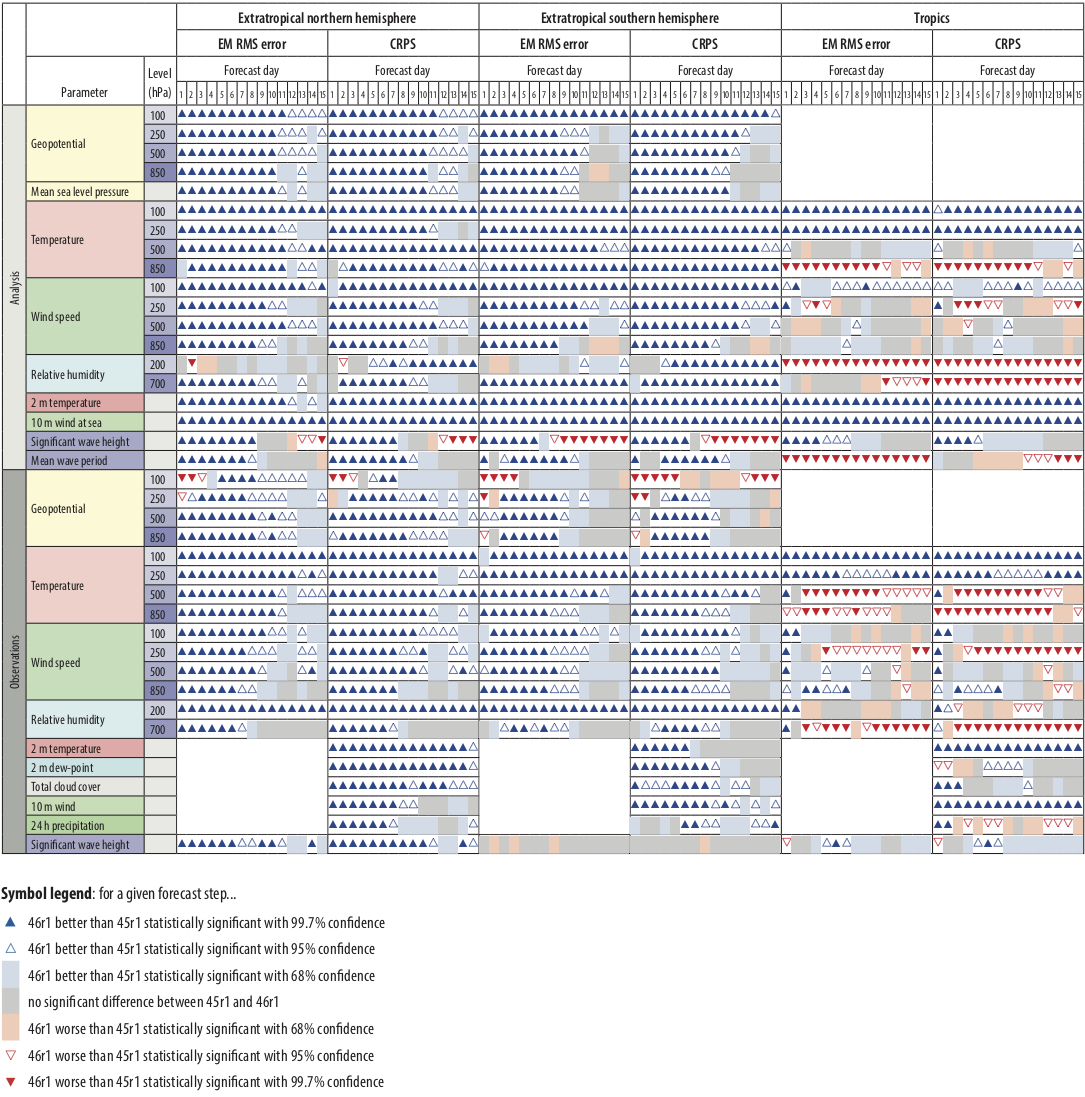
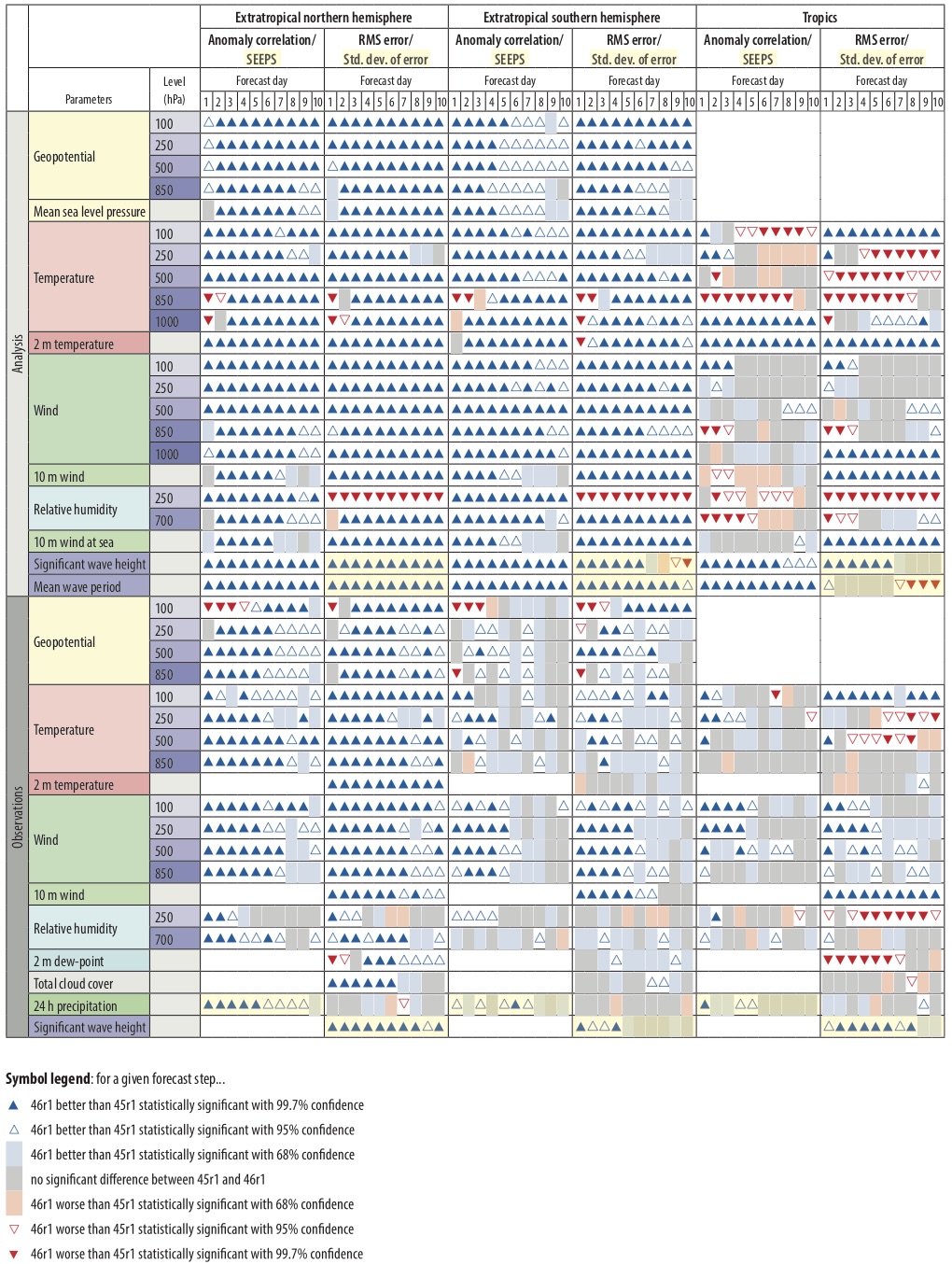
IFS Cycle 46r1 brings substantial improvements in forecast skill for both ENS and HRES (Figures 1 and 2). Medium-range forecast errors in the extratropics are reduced by 1–5% for upper-air parameters and by 0.5–2% for surface parameters. Improvements of this magnitude are seen in verification against both the analysis and observations. In terms of lead time, upper-air improvements amount to a gain of around 2–3 hours. In the tropics, HRES results are predominantly positive, but there are some increases in temperature and humidity errors, mainly seen in verification against the analysis. For temperature, these are due to changes in the analysis and the introduction of the 3D aerosol climatology. ENS results in the tropics are also mixed. In addition to the changes mentioned already, they are affected by a minor reduction in spread (around 1%) due to changes in the deep convection scheme. Wave parameters (significant wave height and mean wave period) in the HRES are improved substantially by 5–10% due to the upgrade in the ocean wave model. Increased wave activity leads to some degradation in wave height at longer lead times in the ENS.
Precipitation forecast skill increases in the extratropics by about 0.5% in the ENS and 1% in the HRES. Other weather parameters, such as 2‑metre temperature and 2‑metre dewpoint, 10-metre wind speed and total cloud cover improve by about 1% in the ENS, and by 0.5–1% in the HRES when verified against observations. In the tropics, slightly reduced spread and increased bias lead to a very small (0.1–0.2%) degradation in ENS precipitation. Scores in the tropics show strong improvements for 2‑metre temperature (4–8% against the analysis both in ENS and HRES, 1–2% against observations in the ENS). Tropical cyclone forecast skill is neutral overall, with a slight reduction in track error, consistent with improved winds in the tropics.


New forecast outputs
An Extreme Forecast Index (EFI) for water vapour flux has been introduced, as well as new EFI products to highlight potential extremes in the extended range (Figure 3). Probabilities for 850 hPa temperature anomalies in terms of standard deviations from the climate average, together with additional probability thresholds for precipitation and near-surface (10 m) wind have been added to support the activities of World Meteorological Organization Members. Ocean fields, including sub-surface data such as the depth of the 20°C isotherm and the average salinity and potential temperature in the upper 300 m, are now also available.
Summary
The implementation of IFS Cycle 46r1 brings us another step closer to the implementation of ECMWF’s ten‑year strategy, which includes two important scientific goals to help improve medium-range forecast skill. One is a more accurate estimation of the initial state and the consistent representation of uncertainty associated with observations and the model. Progress in this direction can be seen in the package of improvements associated with continuous data assimilation; the 50-member EDA and the new consistency between EDA and ENS members; and many other changes. The second is a better representation of physical and chemical processes and of the interactions between different Earth system components. Examples of progress in this area include a faster coupling between radiation, clouds and the surface, because of the more frequent radiation updates; the improvements in the ocean wave model; and many other modelling changes.
Further reading
Ardhuin, F., E. Rogers, A. Babanin, J.-F. Filipot, R. Magne, A. Roland, A. van der Westhuysen, P. Queffeulou, J.-M. Lefevre, L. Aouf & F. Collard, 2010: Semi-empirical dissipation source functions for windwave models: part I, definition, calibration and validation. J. Phys. Oceanogr., 40 (9), 1917–1941.
de Rosnay, P., M. Drusch, D. Vasiljevic, G. Balsamo, C. Albergel & L. Isaksen, 2013: A simplified Extended Kalman Filter for the global operational soil moisture analysis at ECMWF. Q.J.R. Meteorol. Soc., 139, 1199–1213, doi:10.1002/qj.2023.
Hogan, R.J. & A. Bozzo, 2018: A flexible and efficient radiation scheme for the ECMWF model. J. Adv. Modeling Earth Sys., 10 (8), 1990–2008, doi:10.1029/2018MS001364.
Janssen, P. 2017: Shallow water version of the freak wave warning system. ECMWF Technical Memorandum No. 813.
Lang, S., E. Hólm, M. Bonavita & Y. Tremolet, 2019: A 50-member Ensemble of Data Assimilations. ECMWF Newsletter No. 158, 27–29, doi:10.21957/nb251xc4sl.
Lean, P., M. Bonavita, E. Hólm & T. McNally, 2019: Continuous data assimilation for the IFS. ECMWF Newsletter No. 158, 21–26, doi:10.21957/9pl5fc37it.