


For forecasts more than about three days ahead, components of the Earth system that are typically slower to change than the atmosphere become more important. This is true both in terms of their representation in the model and in terms of an accurate specification of the initial conditions on which forecasts are based. Such components include the ocean, sea ice and the land surface and how they dynamically interact with each other and the atmosphere.
One of the goals of coupled data assimilation (Box A) is to make sure that all components of an Earth system model are initialised consistently with one another. If the different components are not mutually consistent, they are sometimes referred to as unbalanced. This lack of balance can lead to fast adjustments in the system in the initial stages of the forecast in a phenomenon known as initialisation shock. Initialisation shock can be reduced by initialising the various components together via coupled data assimilation.
A
What is coupled data assimilation?
In numerical weather prediction, data assimilation is the combination of short-range forecasts with observations to arrive at the best possible estimate of the current state of the Earth system. This estimate, called the analysis, is used to initialise forecasts. In coupled data assimilation, the observations of one Earth system component influence the analysis in other components.
There is enormous variety in the configuration of coupled data assimilation systems, for both technical and scientific reasons. The atmosphere and ocean waves typically change on much shorter timescales than, for example, the ocean subsurface or land surface variables such as soil moisture. Thus, historically, assimilation systems for slower components have been developed independently of those used for the atmosphere. They may work on different operational schedules and may have different assimilation windows (the time during which observations to be used in a data assimilation cycle are made). A further complication is that different assimilation techniques may be used for the various components. It is, however, possible to categorise coupled data assimilation systems by the timing of the influence of observations of one component on the analysis in other components. We refer to strong coupling when there is an immediate impact from observations made in one component on another. If the observation impact from one component on another is lagged, then this is referred to as weak coupling. In uncoupled data assimilation, there is no observation information exchange between different components.


Another goal of coupled data assimilation is to extract as much information as possible from observations and provide it to all relevant parts of the Earth system model. This is because there are many observations that contain information useful to multiple parts of the Earth system. These include, for example, scatterometer data, which contain information on the interface between the Earth surface and the atmosphere. Another example is near-surface observations used in one component that are near a data-sparse region of another component.
Here we describe the form of weakly coupled data assimilation for the atmosphere, the ocean and sea ice implemented operationally in ECMWF’s Integrated Forecasting System (IFS) in June 2018 (IFS Cycle 45r1) and June 2019 (IFS Cycle 46r1). The new system makes it possible to combine information from different Earth system components despite the fact that they have different assimilation windows. Experiments confirm that weakly coupled ocean–atmosphere data assimilation as implemented at ECMWF significantly improves the analysis of atmospheric variables such as temperature and humidity in the tropics and in the polar regions.
ECMWF’s operational setup
The IFS uses models of a range of Earth system components in different combinations for different purposes. The short-range forecasts which are used in the data assimilation system to produce the atmospheric analysis use the atmospheric model, the land model, the lake model, and the wave model. ECMWF’s medium-range to seasonal forecasts, on the other hand, are all produced using those models plus interactive ocean and sea ice models. The latter are the 3-dimensional community ocean model NEMO and the Louvain-la-Neuve 2 (LIM2) sea ice model developed at the Belgian Université Catholique de Louvain. The ocean temperature, salinity, and horizontal currents are initialised separately from the atmosphere using the 3D-Var First Guess at Appropriate Time (FGAT) assimilation technique. The length of the assimilation window varies from 8 to 12 days. In parallel, a sea ice concentration analysis is produced using the same 3D-Var FGAT method. This ocean and sea ice analysis system is known as OCEAN5. Since IFS Cycle 45r1, all of ECMWF’s medium-range forecasts have been fully coupled to OCEAN5 in the tropics and partially coupled in the extratropics.
Observations that are currently assimilated to produce the ocean analysis are in situ profiles of temperature and salinity and satellite-derived sea level anomaly and sea ice concentration observations. For sea-surface temperature (SST), a relaxation is performed towards the OSTIA SST product from the UK Met Office. The ocean and sea ice analysis system requires forcing fields from the atmospheric analyses and forecasts. See Zuo et al. (2018) for full details.
The atmospheric analysis is produced using 4-dimensional variational data assimilation (4D-Var). The land data assimilation component is weakly coupled to the atmosphere. The various components of the land surface are initialised using different methodologies: the snow analysis is produced using a 2D-OI (optimal interpolation) technique, as is the soil temperature analysis, while soil moisture is analysed using a Simplified Extended Kalman Filter. Similar to the land analysis, the wave analysis is weakly coupled to the atmosphere and is produced using 2D-OI.
Tens of millions of observations are processed and used daily. The vast majority of these come from polar-orbiting and geostationary satellites carrying a range of instruments, such as infrared and microwave imagers, scatterometers and altimeters. In addition to satellite observations, there are in situ observations from aircraft, radiosondes and dropsondes, as well as observations from ships, buoys, land-based stations and radar.
The ocean and ice surface conditions need to be supplied to the atmospheric model to drive the 4D-Var data assimilation and the uncoupled short-range forecasts used to produce the atmospheric analysis. Until the implementation of IFS Cycle 45r1 in June 2018, level 4 (L4) gridded products (satellite observations processed to produce complete gridded fields) were used to provide global coverage of sea-surface temperatures and sea ice concentrations to the data assimilation system. The L4 product used was the Operational Sea Surface Temperature and Sea Ice Analysis (OSTIA), a 0.05° resolution dataset that does not use a dynamical model. For SST, OSTIA combines satellite data from the Group for High Resolution Sea Surface Temperature (GHRSST) and in-situ observations to produce a daily analysed field of foundation sea-surface temperature (SST at a depth of about 10 m, not sensitive to the diurnal cycle). Sea ice concentration fields in OSTIA are derived from OSI SAF L3 satellite observations of sea ice concentration.
When using an external L4 product as the lower boundary for the atmosphere, ECMWF’s high-resolution data assimilation system can stand alone, independent of any information from the OCEAN5 analysis. However, OCEAN5 is a different possible source for the lower boundary ocean and ice fields that the atmospheric data assimilation system needs. If these fields are used, the atmospheric and ocean data assimilation systems are combined into a larger, weakly coupled assimilation system.
Weakly coupled data assimilation
When using an external L4 product as the lower boundary condition over the ocean, only those boundary conditions and observations in the atmosphere will influence the atmospheric analysis. This change in atmospheric analysis will lead to a change in the forcing fields by which the ocean analysis is driven. This will lead to a change in the ocean analysis. However, observations of the ocean not used by OSTIA, such as observations of currents, will not influence the atmospheric analysis as no information from the ocean model is propagated back to the atmospheric analysis. This system can be thought of as a ‘one-way’ coupled assimilation system.
To form a ‘two-way’ weakly coupled ocean–atmosphere data assimilation system, ECMWF has begun to use fields from the OCEAN5 analysis as the lower boundary condition for sea ice (since IFS Cycle 45r1) and SST (since IFS Cycle 46r1) in the atmospheric data assimilation system. This means that observations of the ocean and the sea ice which previously only influenced the ocean analysis now also modify the atmospheric analysis via the lower boundary conditions. The effect is not immediate within a given assimilation cycle but is delayed. The reason for this is that the OCEAN5 near-real-time analysis only produces a single analysis every day. The atmospheric analysis must wait for the ocean analysis fields, valid at the end of the day, to be produced to force the next day’s atmospheric analyses. Hence, we categorise this as a weakly coupled data assimilation system for the ocean, sea ice and the atmosphere.
The analysis of SST and sea ice concentration from OCEAN5 may not always be better than the OSTIA product. Indeed, there are known deficiencies in the OCEAN5 analysis that would lead to degradations in forecast performance if left unmitigated. For example, in the extratropics the position of western boundary currents such as the Gulf Stream is known to be less accurate in OCEAN5 than in OSTIA.
This problem has been addressed within the model by using a ‘partial-coupling’ approach, in which the tendencies (the model evolution from its initial conditions) rather than the absolute values of SST are passed to the atmosphere. Since the ocean model in OCEAN5 has greater effective resolution in the tropics than the extratropics, the partial coupling is only required at higher latitudes (> 25°), where the ocean model is unable to resolve eddies.
In IFS Cycle 46r1, the SST in the atmospheric analysis is aligned with that used to initialise the coupled forecast, which is SST from the OCEAN5 analysis in the tropics, smoothly transitioned to the OSTIA SST in the extratropics.
Evaluation
To assess the impact of the weakly coupled ocean–atmosphere configuration compared to the previous use of L4 products for the lower boundary conditions in the atmospheric data assimilation system, two experiments were conducted: a control experiment (CTR) which does not use any weakly coupled assimilation, and a second experiment (EXP) with weakly coupled assimilation in both sea ice and sea-surface temperature.
Both experiments are based on IFS Cycle 45r1 at the operational high-resolution grid spacing of 9 km (TCo1279). They cover the period 9 June 2017 to 21 May 2018. From each analysis, a coupled ocean–atmosphere forecast is produced and is compared against the respective analysis. When a coupled forecast is initialised, the atmospheric lower boundary conditions are replaced by those coming from the ocean and sea ice analysis. If, as is the case here, the ocean and sea ice analyses are similar, then weakly coupled data assimilation does not change the coupled forecasts dramatically. However, the results show that there are differences between EXP and CTR in the atmospheric analysis at the interface between the ocean/sea ice and the atmosphere, and that these propagate vertically into the troposphere. The extra information provided by the weakly coupled system thus aligns the atmospheric analysis more closely with coupled forecasts, at least in the short range.


In the Arabian Sea, there is evidence of improvements in the analysis of other variables, such as low-level winds and significant wave height (not shown). This indicates that weakly coupled data assimilation improves the position of the summer monsoon, which is known to be difficult to predict well. The regions of positive impact in the Atlantic and the equatorial Pacific tend to have high cloud cover. This persistent cloud cover makes observing the SST from satellites difficult. The use of the ocean model within the OCEAN5 analysis system seems to be able to effectively fill the observational gap.
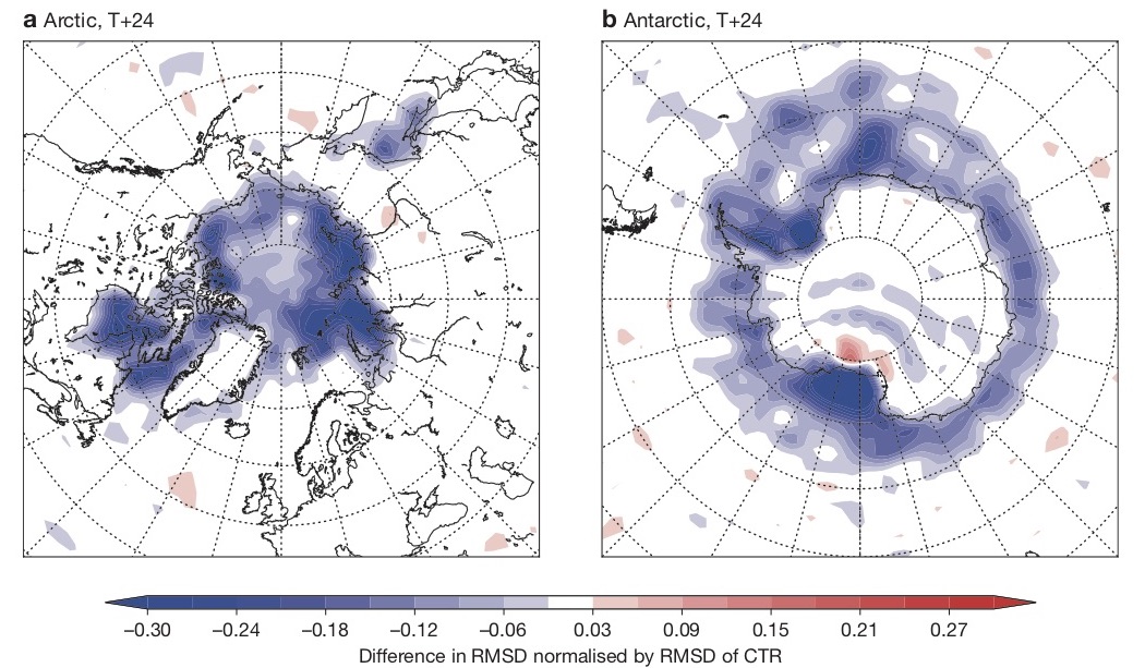
In the polar regions, we see significant reductions in the differences between coupled short-range forecasts and the analysis due to weakly coupled assimilation. Figure 3 shows that the improvements due to sea ice are not confined to the ice edge but encompass the entire extent of sea ice cover.
A detailed look at the spatial distribution of sea ice in the Baltic Sea (Figure 4) shows that weakly coupled data assimilation captures the structures seen in the manual ice chart much better than the L4 product. Note that because of the geography and coastal contamination of satellite observations, this is a particularly challenging area for sea ice concentration analyses. The use of the background information coming from the dynamical model leads to a much more realistic spatial distribution of the ice field.

Conclusions and future plans
Weakly coupled data assimilation enables components of the Earth system with different timescales and assimilation methods to be linked together. As an alternative to using purely observation-based L4 products for the lower boundary of the atmosphere, with their associated delays, weakly coupled data assimilation enables dynamical models of the ocean and sea ice to fill in the gaps in observations and to propagate fields to the appropriate time. It improves the match between coupled forecasts and ECMWF’s analysis in regions near the interface between the atmosphere and the ocean/sea ice and up to an altitude of about 700 hPa.
In the future, we will look to build on the currently operational system to couple more ocean variables to the atmospheric analysis. For example, a weakly coupled data assimilation system that has knowledge of ocean currents should be able to better make use of scatterometer data, and it should enable improvements in wave modelling.
The system described in this article represents the first steps in operational coupled ocean–atmosphere assimilation at ECMWF. It represents the baseline for further coupled ocean–atmosphere data assimilation developments, which will rely on a progressive implementation of combined weak and outer-loop coupling. In outer-loop coupling, coupled model trajectories are used within the data assimilation system whilst the linearised trajectories remain uncoupled (see Schepers et al., 2018). This will give more immediate impact across the various Earth system components for the benefit of medium-range and extended-range forecasts.
Further reading
Browne, P. A., P. de Rosnay, H. Zuo, A. Bennett & A. Dawson, 2019: Weakly Coupled Ocean-Atmosphere Data Assimilation in the ECMWF NWP System. Remote Sensing, 11 (234), 1–24, doi:10.3390/rs11030234.
Schepers, D., E. de Boisséson, R. Eresmaa, C. Lupu & P. de Rosnay, 2018: CERA-SAT: A coupled satellite-era reanalysis, ECMWF Newsletter No. 155, 32–37.
Zuo, H., M.A. Balmaseda, K. Mogensen & S. Tietsche, 2018: OCEAN5: the ECMWF Ocean Reanalysis System and its Real-Time analysis component. ECMWF Technical Memorandum No. 823.