
Accurate weather predictions are not possible without an accurate specification of the initial state of the Earth system. To this end, billions of observations of the Earth system are made every day. Data assimilation combines many of those observations with model information to arrive at a full set of initial conditions called the analysis. In the current ECMWF operational configuration, by the time the analysis is complete, the most recent observations that have gone into producing it are almost two hours old. This article presents a revised configuration of ECMWF’s 4D-Var data assimilation system designed to allow the analysis to benefit from more recent observations. In the new, more continuous framework, we are able to assimilate observations taken around one and a half hours later than in the current system. In addition, more accurate albeit more time-consuming data assimilation configurations can be accommodated inside the operational schedule, providing scope for further improvements in analysis and forecast skill in upcoming cycles. The new data assimilation configuration has been found to improve forecast quality significantly. It is due to be implemented in the next upgrade of ECMWF’s Integrated Forecasting System (IFS Cycle 46r1), scheduled for 2019.
Operational schedule
For an observation to be useful for numerical weather prediction (NWP), it must be delivered in a timely manner. To allow for the inevitable delay between the time that an observation is made and the time at which it is available for use, most operational centres (including ECMWF) structure their operational data assimilation (DA) and forecasting schedule in two distinct phases. First, there is a data collection phase, during which we wait for the observations to arrive. After a predefined data cut-off time, the computation of the analysis and the forecast begins (see Figure 1).

Since the time at which forecasts are issued to users is usually fixed, the choice of the data cut-off time involves a trade-off between two competing requirements: allowing more time for observations to arrive (which should lead to a more accurate analysis and hence better forecasts); and allowing more time for the DA and forecast computations to be completed (which should also result in a more accurate analysis and better forecasts through, e.g., more sophisticated algorithms, increased resolution, etc.).
In ECMWF’s current operational schedule, the DA computations do not begin until an hour after the end of the assimilation window (the time during which observations to be used in a data assimilation cycle are made). For example, computing the 00 UTC analysis with a 21 to 03 UTC assimilation window starts at around 04 UTC. The observation quality control and DA computations take about an hour to complete. This means that by the time the analysis has been produced, the most recent observations that went into producing it are about two hours old.
Current DA configuration
Since its operational implementation in the late nineties (Rabier et al., 2000), ECMWF has used incremental 4D-Var as its atmospheric DA algorithm. Incremental 4D-Var (Courtier et al., 1994) works by iteratively minimising a cost function to achieve the best possible fit between a short-range forecast (the background) on the one hand and observations on the other. The model and the observation operators are repeatedly linearised around a progressively more accurate model trajectory solution. These relinearisations are called outer loops. The outer loop mechanism has recently been shown to be one of the key drivers of analysis and forecast accuracy in the IFS (Bonavita et al., 2018). It is, however, a strictly sequential algorithm in the sense that successive linearisations and minimisations need to be performed one after the other for the procedure to converge. This imposes rather stringent limits on the complexity of the incremental 4D-Var configurations that can be run within ECMWF’s operational time constraints.
A partial answer to the time-constraint problems described above was provided with the introduction of the early-delivery suite at ECMWF (Haseler, 2004). As the data cut-off is only one hour after the end of the assimilation window, many observations have not arrived by this time. A second, ‘delayed cut-off’ assimilation cycle is run which assimilates all observations that have arrived within 4 hours of the end of the assimilation window. The delayed cut-off cycle is thus able to make use of a much larger number of observations and thus to provide an analysis (called the long-window data assimilation analysis, or LWDA analysis) of higher accuracy than the one produced by the early-delivery suite. The LWDA analysis is then used to produce a short-range forecast (the background) which is used in the next early-delivery cycle. In this way, late-arriving observations can benefit the quality of the following analysis through a more accurate background. However, the limitations on the complexity of the 4D-Var algorithm that can be used in operational practice remain.
Continuous DA configuration
The general idea of a continuous DA system based on 4D-Var is not new. Variations on it were proposed in the mid-nineties (Järvinen et al., 1996; Pires et al., 1996) and even used operationally for a while at Environment Canada (Gauthier et al., 2007). In a continuous DA framework, we do not wait for all the observations to arrive before starting the analysis computations. In effect, the computation phase overlaps with the data collection phase. We call these schemes ‘continuous DA’ as, in principle, they can be run continuously in the operational schedule with new observations being fed to the assimilation system as they arrive. Motivated by the aim of allowing more recent observations into the analysis, a variant of this concept will be introduced in IFS Cycle 46r1.
The incremental 4D-Var outer loop provides a convenient mechanism by which newly arrived observations can be introduced into the system after the assimilation has started. The idea is that, instead of stopping observations entering the 4D-Var analysis after a fixed cut-off time, new observations are allowed in between successive outer loops (Figure 2). As each outer loop takes about 15 minutes to complete, in the new continuous DA we have extended the effective cut-off time by around 25 minutes.

From an algorithmic point of view, instead of solving a fixed minimisation problem, we solve a series of slightly different minimisation problems as the number of observations increases from one outer loop to the next.
To fully benefit from the later cut-off time, we have extended the assimilation window of the early-delivery analysis from 6 hours to 8 hours. This ensures that it extends right up to the time at which the DA runs. In our current system, the 00 UTC analysis has an assimilation window from 21 UTC to 03 UTC. The DA for this cycle begins after the 04 UTC cut-off time. Many observations taken in the 03 to 04 UTC period have already arrived by this time, but are not used. By extending the assimilation window by two hours to 05 UTC, we can assimilate these very valuable observations and later ones, enabling the state to be constrained by observations a further one and a half hours into the forecast.
All the newly arrived observations need to also go through quality control. This is achieved by performing observation screening in each outer loop on all available observations (not just those that have arrived since the previous outer loop). An advantage of this approach is that the quality control is performed against a more accurate model trajectory than the previous model background, which should lead to improved screening decisions.
Our previous operational schedule was based upon a trade-off between the time allocated to the arrival of observations on the one hand and the time allocated to the DA computations on the other. In the continuous DA framework, we no longer need to wait until 04 UTC to begin the 00 UTC analysis, as later-arriving observations will be captured in successive 4D-Var outer loops. As a result, we are now able to start the 4D-Var computations earlier. In Cycle 46r1, we will start the assimilation around 10 minutes earlier and use this time to increase the number of outer loops from three to four. Even this simple change has been shown to have a statistically significant positive impact on analysis and forecast skill (Bonavita et al., 2018).
The changes described so far are applied to the time-critical early-delivery assimilation. As the LWDA cycles (which provide the background for the early-delivery assimilation) already have a very late observation cut-off time, there is no need to use the continuous DA approach here, and the length of the assimilation window is kept at 12 hours. The only change to the LWDA cycles is the addition of an extra outer loop to further improve the accuracy of the background.
|
Outer Loop |
Number of observations in EXP relative to CTRL |
|---|---|
| 1 | 101% |
| 2 | 107% |
| 3 | 110% |
| 4 | 114% |
TABLE 1 Number of observations used in each outer loop of 4D-Var in a six-month continuous DA experiment (EXP), relative to the number of observations used in the current operational setup (CTRL).
|
Outer Loop |
Average number of iterations in CTRL |
Average number of iterations in EXP |
| 1 | 31.5 | 31.1 |
| 2 | 29.9 | 31.2 |
| 3 | 30.4 | 28.8 |
| 4 | - | 29.6 |
TABLE 2 Average number of iterations required to achieve convergence in the 4D-Var DA system in a six-month experiment using the operational setup (CTRL) on the one hand and continuous DA on the other (EXP).
Results
In the new early-delivery assimilation, the number of observations increases in each outer loop. In an experiment covering six months (EXP), the first outer loop had slightly more observations than the first outer loop in an experiment using the current system (CTRL), even though it has an earlier cut-off (see Table 1). The reason is that the assimilation window in EXP is longer than in CTRL. Overall, the continuous DA configuration uses around 14% more observations than the current early-delivery DA. An example of the geographic distribution of the extra observations assimilated in a single cycle using continuous DA is shown in Figure 3.
Before running these experiments, an initial concern was that introducing new observations at each outer loop changes the minimisation problem being solved. It was thought that this might make the preconditioning techniques used to accelerate the convergence of 4D-Var less effective and might even cause numerical problems. Table 2 shows that there were no issues in this respect. A possible explanation is that the relatively small change in observation counts from one outer loop to the next (up to about 6% of total observation numbers) does not change the topology of the cost function significantly. Another reason is that the preconditioners represent only broad, large-scale features of the underlying cost function and thus tend to be insensitive to small, localised changes in observation coverage.


In general, medium-range forecast scores are improved by around 2% at day 3 in the extratropics for most variables. Examples of the improvements can be seen in Figures 4 and 5. In the tropics, 500 hPa wind shows a statistically significant improvement out to day 9. The improvements are widespread and geographically fairly uniform (Figure 6). These results are consistent with an improvement in predictability of around 2 to 3 hours. This comes from the extra one and a half hours of observational data, combined with the improved assimilation enabled by the extra outer loop.


Observation timeliness
Up until now, any observations that arrive within 1 hour of the time that they were made will be processed in the early-delivery cycle. With a continuous DA configuration, the analysis quality becomes more responsive to changes in the timeliness of observation delivery.
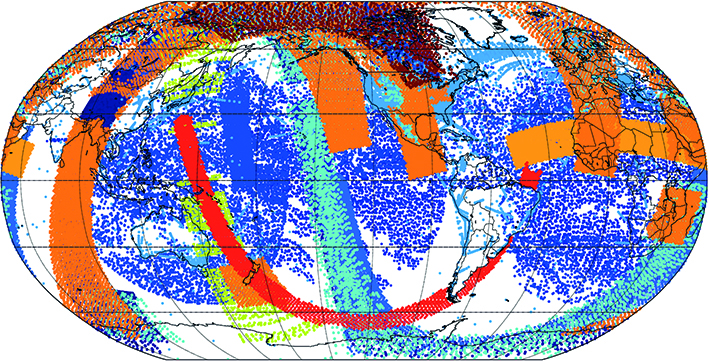
Figure 7 shows an example of the geographical distribution of observations made between 04:00 and 04:25 UTC (towards the end of the extended 4D-Var assimilation window) and assimilated in the continuous DA configuration. The coverage is far sparser than for observations made during earlier parts of the assimilation window. Only observations which are delivered within at most 25 minutes of the observation time will be used in this period. In this example, we see many conventional observations, including some AMDAR reports from aircraft over the North Atlantic, Europe and North America. In addition, data from polar-orbiting satellites as they downlink data over the ground stations in the polar latitudes and at local reception stations of the Direct Broadcast Network (DBNet) can be seen.
It is easy to see how improving the timeliness of all observation types would increase the coverage at the end of the window, further constraining the analysis and leading to increased predictability in the forecasts. The DBNet initiative, coordinated by the World Meteorological Organization, is an example of how this can be achieved in a very cost-effective way (http://www.wmo.int/pages/prog/sat/rars_en.php). It uses a network of ground stations that process local satellite overpasses in a globally consistent way and can thus achieve very good timeliness. Expanding such initiatives will bring even greater benefits in the new continuous DA framework. In the continuous DA configuration, we will still be able to use less timely data, but improved timeliness will substantially increase the number of observations that can be used.
Future possibilities
Continuous DA opens the door to exciting new avenues of research and new configurations of our system. It makes it possible for significantly more expensive, but correspondingly more accurate 4D-Var configurations to fit into the operational schedule. In Cycle 46r1, we take advantage of this by starting the assimilation 10 minutes earlier to accommodate an extra outer loop. However, this could be taken further in upcoming cycles. For example, the possibility of running higher-resolution minimisations or using stricter convergence criteria is currently being explored. Taking this development to its logical extreme, we can envisage the possibility that, one day, our assimilation system could run quasi-continuously with new observations being drip-fed into the system as they arrive, progressively refining our analyses.
Conclusions
The current Global Observing System (GOS) produces a continuous flow of observations that can be used to improve the initial conditions and forecast skill of NWP systems. The pre-processing and initial quality control of these observations is also transitioning at ECMWF towards a near-continuous framework in the context of the Continuous Observation Processing Environment (COPE) project. The continuous data assimilation system described in this article represents a first step at ECMWF to better exploit the steady stream of available observations and, more generally, to adapt the ECMWF data assimilation system to the changing characteristics of the GOS. An important by-product of this development is the fact that it makes more time available for DA computations. This will enable us to introduce more effective 4D-Var configurations in operations while maintaining the same product dissemination schedule and reducing pressure on the time-critical part of the operational suite. Further improvements are possible in this area (e.g. increasing the resolution of the minimisations, more accurate linearisation states, etc.) and are currently being explored.
In the continuous DA framework, we can assimilate observations taken around one and a half hours later than in the current system, as well as delayed observations that would previously have arrived after the cut-off time. In addition, the extension of the assimilation window up to the cut-off time makes the quality of our forecasts more responsive to changes in the timeliness of observation delivery.
Experiments with this first version of continuous DA reflect the benefits of being able to assimilate more observations and producing a more accurate 4D-Var analysis, with predictability gains of two to three hours for typical skill scores.
As important as these forecast improvements are, a possibly more consequential change is the new possibilities that the continuous DA framework offers for the evolution of the ECMWF DA system. Conceptually it is easy, for example, to extend the continuous DA setup towards an assimilation system running continuously ‘in the background’ and continuously providing updated estimates of the initial conditions of the Earth system based on the steady stream of incoming observations.
Further reading
Bonavita, M., P. Lean & E. Holm, 2018: Nonlinear effects in 4D-Var, Nonlinear Processes in Geophysics, 25, 713–729.
Courtier, P., J.-N. Thépaut & A. Hollingsworth, 1994: A strategy for operational implementation of 4D-Var, using an incremental approach, Q. J. Roy. Meteor. Soc., 120, 1367–1387, https://doi.org/10.1002/qj.49712051912.
Gauthier, P., M. Tanguay, S. Laroche, S. Pellerin & J. Morneau, 2007: Extension of 3DVAR to 4DVAR: Implementation of 4DVAR at the Meteorological Service of Canada, Mon. Wea. Rev., 135, 2339–2354.
Haseler, J., 2004: Early-delivery suite. ECMWF Technical Memorandum No. 454. https://www.ecmwf.int/en/elibrary/9793-early-delivery-suite
Järvinen, H., J.-N. Thépaut & P. Courtier, 1996: Quasi-continuous variational data assimilation, Q. J. Roy. Meteor. Soc., 122, 515–534.
Pires, C., R. Vautard & O. Talagrand, 1996: On extending the limits of variational assimilation in nonlinear chaotic systems, Tellus A, 48, 96–121.
Rabier, F., H. Järvinen, E. Klinker, J.-F. Mahfouf & A. Simmons, 2000: The ECMWF operational implementation of four-dimensional variational assimilation. Part I: Experimental results with simplified physics. Q. J. Roy. Meteor. Soc., 126, 1143–1170.