Lightning is one of the most spectacular phenomena in the atmosphere. It can affect the environment by triggering wildfires. It can also disrupt air traffic and airport activities such as refuelling; cause power supply outages or power surges that can harm electronic equipment; damage buildings; and even lead to fatalities. Lightning also plays a significant role in the production of mid-tropospheric nitrogen oxides, which in turn influence the ozone budget.
Lightning is usually associated with intense convective activity and most commonly occurs in the troposphere. Somewhat fainter electrical luminous events that extend well above the top of convective clouds into the stratosphere and beyond, such as sprites, elves and blue jets, have started to be documented in recent years but their impact on human activities is negligible. Occasionally lightning can also be triggered in the ash cloud of volcanic eruptions. However, the focus of this article is on lightning produced by convection inside the troposphere, which is by far the most common cause.
ECMWF has developed a lightning parametrization that is expected to provide global predictions of lightning activity operationally from mid-2018. Experiments have shown that ECMWF ensemble forecasts (ENS) for lightning can have useful skill to at least day 3, while a good agreement with observations can be achieved in deterministic forecasts on temporal and spatial scales above 6 hours and 50 km.
Work is under way to enable the model to distinguish between cloud-to-ground and intra-cloud lightning. The possibility of assimilating observations from lightning imagers on new geostationary satellites is also being investigated.
Physics of lightning
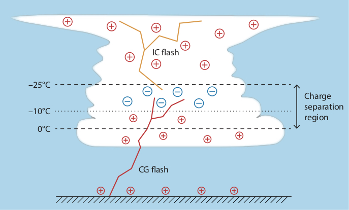
From a physical point of view, convective lightning discharges occur in response to a local build-up of an atmospheric electric field. This field in turn results from the separation of positive and negative electric charges inside neighbouring convective regions. A highly simplified schematic of the typical tripole structure of electric charges inside a deep convective cloud is shown in Figure 1. A predominantly negatively charged layer is found between roughly –25°C and –10°C, below a deep positively charged layer extending toward the top of the cloud, and above another positively charged but shallower layer extending between the –10°C level and the base of the cloud. A more detailed description of the electrification mechanism inside convective clouds is given in Box A.
As illustrated in Figure 1, lightning flashes can be categorised as cloud-to-ground (when the electric discharge takes place between the cloud and the Earth’s surface) or intra-cloud (when the discharge occurs between two cloud regions containing oppositely charged hydrometeors). These two types of lightning flashes will hereafter be referred to as CG and IC, respectively. The fraction of IC flashes is around 80% on average, although this percentage can fluctuate between 30% and 100% according to geographical location and thunderstorm characteristics. It is also worth noting that CG flashes are often characterised by much stronger peak currents (i.e. higher energy) than IC flashes.
Lightning observations
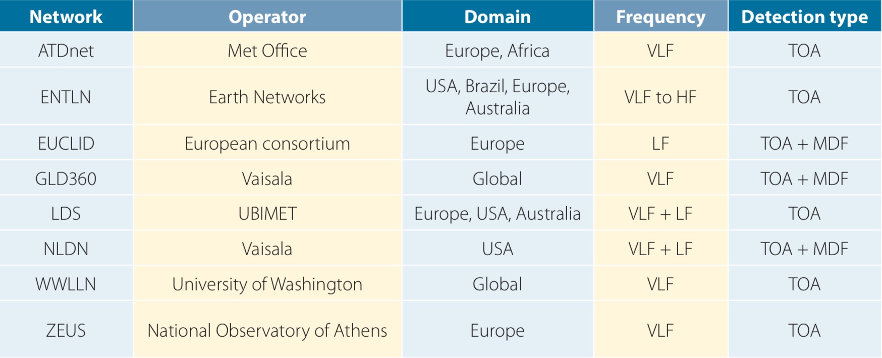
Continuous observations of lightning with wide spatial coverage are currently available from two main sources. First, several global, continental or national-scale networks of ground-based lightning sensors provide continuous monitoring of the location and, in some cases, of the intensity of lightning activity. The sensors work by detecting the electromagnetic emissions (so-called ‘sferics’) produced by individual lightning strokes. Most networks analyse sferics at either very low frequency (VLF; 3–30 kHz) or low frequency (LF; 30–300 kHz), which allows their detection over a range of several hundred kilometres. Some of them can also operate at high frequency (HF; 3–30 MHz) or very high frequency (VHF; 30–300 MHz), although at such wavelengths the detection range is usually reduced. Using a method based on time of arrival (TOA) or magnetic direction finding (MDF) or both, the information from several sensors must be combined to locate individual lightning strokes with useful accuracy (a few kilometres or less). An additional estimate of the peak current of each stroke can also be obtained. Table 1 gives a non-exhaustive list of the largest networks currently in use and their characteristics, with a particular focus on Europe.
A
How lightning is generated
The typical electric charge distribution shown in Figure 1 is the result of charge separation. Charges are separated during collisions between various types of hydrometeors with very different fall speeds, especially graupel or hail particles on the one hand and lighter ice particles or liquid water droplets on the other. Depending on whether the ambient temperature is higher or lower than about –10°C, graupel/hail particles involved in such collisions become positively or negatively charged, respectively. Both non-inductive and inductive processes are thought to be responsible for charge separation. By their nature, inductive processes require the existence of a sufficiently strong electric field in the environment and can thus only become effective after a preliminary electrification due to non-inductive processes. Once the electric field produced by charge separation locally exceeds a certain threshold, a lightning discharge can be triggered, which cancels out some of the charges. This in turn reduces the ambient electric field. A typical lightning discharge involves the preliminary ionisation of a channel that jerkily propagates through the atmosphere (a so-called leader), which can take several hundred milliseconds. Once the leader attaches to either the ground or another, oppositely charged part of the cloud, one or several strokes propagate through the ionised channel for a few microseconds each, producing very intense electric currents (typically 10 to 100 kA) and extremely high temperatures (typically 10,000 to 30,000 K). These successive strokes are the components of what one visually identifies as a lightning flash. The total duration of a flash usually remains well below a second.
A major limitation of ground-based sensors is that their detection efficiency is often much lower for IC than for CG lightning strokes, due to the lower energy usually released by the former. Furthermore, detection efficiency and stroke location accuracy depend on the number of lightning sensors covering any particular area.
The other main source of lightning observations is space-borne imagers, which can detect the optical signature of lightning events at a wavelength of 777.4 nm (oxygen emission line). The identification of lightning pulses requires the continuous monitoring of the background scene and the detection efficiency is higher at night than during the day, when the background is brighter. Unlike ground-based sensors, satellite lightning imagers can identify both CG and IC lightning strokes with equal efficiency. The Optical Transient Detector (OTD; 1995–2000) and the Lightning Imaging Sensor (LIS; 1998–2013) were the first lightning imagers and were installed on board low-Earth-orbit (LEO) satellites. In 2017, a spare LIS instrument was installed on the International Space Station (ISS) for at least two years. More importantly, the new generation of geostationary satellites GOES-16 and GOES-17 (USA) and FY-4A (China) have all been equipped with lightning imagers (GLM and LMI, respectively).European Meteosat Third Generation geostationary satellites will have a similar lightning imaging capability (MTG-LI; from 2021). Once operational, and in contrast with previous LEO instruments, these new geostationary imagers will provide unprecedented observational coverage in both time (20-second refresh rate) and space (full Earth disc) at a resolution of around 8 km, with a flash detection efficiency greater than 70% and a location error better than 5 km.
%3Cstrong%3E%20Table%201%E2%80%82%3C/strong%3E%20List%20of%20wide-scale%20networks%20of%20ground-based%20lightning%20sensors%20and%20their%20main%20characteristics.%20%3Cstrong%3E%20VLF%20%3C/strong%3E%20=%20very%20low%20frequency,%20%3Cstrong%3E%20LF%20%3C/strong%3E%20=%20low%20frequency,%20%3Cstrong%3E%20HF%3C/strong%3E%20%20=%20high%20frequency,%20%3Cstrong%3E%20TOA%20%3C/strong%3E%20%20=%20time%20of%20arrival,%20%3Cstrong%3E%20%20MDF%20%3C/strong%3E%20=%20magnetic%20direction%20finding. Table 1 List of wide-scale networks of ground-based lightning sensors and their main characteristics. VLF = very low frequency, LF = low frequency, HF = high frequency, TOA = time of arrival, MDF = magnetic direction finding.
%3Cstrong%3E%20Figure%202%E2%80%82%3C/strong%3E%20Annual%20mean%20flash%20densities%20from%20the%20LIS/OTD%20satellite%20climatology. Figure 2 Annual mean flash densities from the LIS/OTD satellite climatology.
Climatology of lightning
A widely used global climatology of lightning activity at 0.5° resolution was produced by Cecil et al. (2014) by combining satellite lightning imager observations from the OTD instrument (1995–2000) and the LIS instrument (1998–2010). Figure 2 shows annual mean lightning flash densities from the LIS/OTD climatology. The overall mean lightning flash density of 2.86 per km2 per year means that an average of 46.2 flashes are observed every second around the globe. Figure 2 highlights the world’s major lightning hotspots: the Congo Basin (in excess of 50 flashes/km2/year over a large area and locally in excess of 150), Colombia, Malaysia, the region south of the Himalayas and Florida. It also clearly shows the predominance of lightning over land in the overall mean. Possible explanations proposed for the much weaker lightning activity over oceans include the weaker convective updraughts and/or the lower aerosol concentrations in the marine planetary boundary layer (hence larger liquid droplets, heavier warm-phase precipitation and less graupel and hail available for charge separation). Of course, strong variations in lightning activity can be observed on the seasonal timescale (not shown), especially over extratropical land regions.
B
Lightning parametrization
In the version planned for operational implementation in IFS Cycle 45r1, the lightning parametrization does not discriminate between CG and IC flashes. It calculates total (i.e. CG+IC) flash density fT (in flashes/km2/day) as
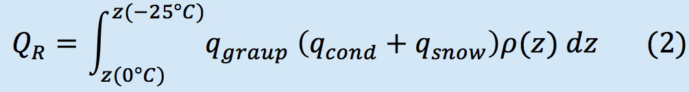
where α is a tunable coefficient, currently set to 37.5 to match the annual global mean flash rate from the LIS/OTD climatology. The variable zbase is the convective cloud base height (in km). The term QR denotes a proxy for the charging rate resulting from the collisions between graupel particles and other types of hydrometeors inside the charging layer and is computed as
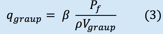
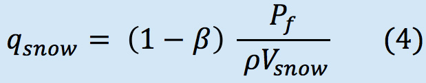
In Equation (2), qcond, qgraup and qsnow denote the amount of convective cloud condensate, graupel and snow, respectively (in kg/kg), while ρ(z) is the ambient air density (in kg/m3) at altitude z. The amount of graupel and snow at each model level is diagnosed from the convective frozen precipitation flux Pf by writing
where β is set to 0.7 over land and 0.45 over sea, while constant fall speeds Vgraup and Vsnow for graupel and snow are assumed to be 3.0 and 0.5 m/s, respectively.
Parametrization of lightning in the IFS
A parametrization of lightning has been developed for ECMWF’s Integrated Forecasting system (IFS) with two main purposes in mind: predicting lightning, i.e. the diagnosis of lightning activity for forecasting applications, and the assimilation of lightning observations, which might bring an improvement in the quality of ECMWF’s atmospheric analyses and forecasts.
The parametrization estimates total (i.e. CG+IC) lightning flash densities using information about convective hydrometeor amounts, convective available potential energy (CAPE) and convective cloud base height, which are already diagnosed by ECMWF’s convection scheme. More details on its formulation can be found in Box B as well as in Lopez (2016). The scheme has been calibrated to match the annual mean flash densities from the LIS/OTD satellite climatology of Cecil et al. (2014) shown in Figure 2. A linearised version of the lightning parametrization has also been coded and tested, since this will be an essential ingredient of the future 4D-Var assimilation of lightning observations.
%3Cstrong%3E%20Figure%203%E2%80%82%3C/strong%3E%20Annual%20mean%20lightning%20flash%20densities%20from%20(a)%20the%20LIS/OTD%20satellite%20climatology%20and%20(b)%20ten%20one-year-long%20IFS%20model%20runs,%20both%20at%2080%20km%20resolution.%20Note%20that%20panel%20(a)%20shows%20the%20same%20field%20as%20Figure%202,%20but%20at%20a%20coarser%20resolution. Figure 3 Annual mean lightning flash densities from (a) the LIS/OTD satellite climatology and (b) ten one-year-long IFS model runs, both at 80 km resolution. Note that panel (a) shows the same field as Figure 2, but at a coarser resolution.
From IFS Cycle 45r1, forecasts of both instantaneous and time-averaged total lightning flash densities will be available to ECMWF users.
Validation of the lightning parametrization
Figure 3 compares the annual mean total lightning flash densities computed from a series of ten 1-year-long IFS model runs at 80 km resolution with the LIS/OTD climatology. Overall, the spatial distribution of lightning activity from the model agrees well with observations. This is also true of its intensity, with the exception of the Congo Basin, where the extremely high climatological values are clearly underestimated in the model.
As an example of the performance at higher spatial resolution, Figure 4 compares time series of daily mean lightning flash densities over Europe from IFS deterministic short-range (0–24 h) forecasts at 18 km resolution with ground-based observations from UBIMET LDS (see Table 1) during the summer of 2015. On the continental scale, the day-to-day variations of model lightning agree quite well with those of UBIMET observations. The results are expected to be at least as good for the current highest operational resolution of 9 km. Naturally, this level of agreement is expected to degrade for smaller averaging times and areas. This is illustrated in Figure 5, which shows how the mean correlation between maps of IFS and UBIMET lightning flash densities varies with the averaging scale in both time (from 1 h to 24 h) and space (from 0.15° to 5°). Figure 5 suggests that accurately forecasting lightning on a scale of a few tens of kilometres and within an hour is still very challenging with the IFS. However, this is also true of other aspects of convective activity, such as precipitation (not shown). Model versus UBIMET lightning correlations do increase noticeably as the time and space constraints are relaxed (up to 0.75 correlation for daily averages over 5° boxes). Similar results are found against other observing networks (not shown).
In addition, the mean diurnal cycle of lightning activity in deterministic forecasts can be validated against ground-based lightning observations. To overcome the variable detection efficiency of ground-based networks, the observed and modelled lightning diurnal cycles are both normalised between 0 and 1, so as to focus on the lightning activity timing. As an example, Figure 6 shows mean diurnal cycle plots from the IFS and from three European ground-based networks of lightning sensors (ATDnet, EUCLID and UBIMET LDS) over the summer of 2015. The figure indicates that the simulated lightning activity peaks at around 1500 UTC, which is about an hour ahead of the observed peak of activity. Furthermore and more importantly, lightning in the model tends to decay rather rapidly in the late afternoon, while observed lightning remains active until the middle of the night. This behaviour of simulated lightning is consistent with previous diagnostics based on the comparison of precipitation forecasts with ground-based radar observations. Past development efforts have brought the triggering of convection in the IFS into line with observations. However, simulated convective activity still vanishes too soon.
%3Cstrong%3E%20Figure%204%E2%80%82%3C/strong%3E%20Time%20series%20of%20daily%20mean%20lightning%20flash%20densities%20from%20IFS%20short-range%20forecasts%20at%2018%20km%20resolution%20and%20from%20UBIMET%20LDS%20ground-based%20observations%20over%20Europe%20during%20the%20summer%20of%202015. Figure 4 Time series of daily mean lightning flash densities from IFS short-range forecasts at 18 km resolution and from UBIMET LDS ground-based observations over Europe during the summer of 2015.
%3Cstrong%3E%20Figure%205%E2%80%82%3C/strong%3E%20Mean%20map-to-map%20correlation%20for%20lightning%20flash%20densities%20between%20IFS%20short-range%20forecasts%20and%20ground-based%20observations%20from%20UBIMET%20LDS%20for%20different%20averaging%20periods%20as%20a%20function%20of%20averaging%20spatial%20resolution%20over%20Europe%20during%20the%20summer%20of%202015.%20 Figure 5 Mean map-to-map correlation for lightning flash densities between IFS short-range forecasts and ground-based observations from UBIMET LDS for different averaging periods as a function of averaging spatial resolution over Europe during the summer of 2015.
%3Cstrong%3E%20Figure%206%E2%80%82%3C/strong%3E%20Mean%20diurnal%20cycle%20of%20lightning%20activity%20(normalised%20between%200%20and%201)%20from%20IFS%20short-range%20forecasts%20at%2018%20km%20resolution%20and%20from%20three%20European%20ground-based%20networks%20of%20lightning%20sensors%20(ATDnet,%20EUCLID%20and%20UBIMET%20LDS)%20over%20the%20summer%20of%202015. Figure 6 Mean diurnal cycle of lightning activity (normalised between 0 and 1) from IFS short-range forecasts at 18 km resolution and from three European ground-based networks of lightning sensors (ATDnet, EUCLID and UBIMET LDS) over the summer of 2015.
%3Cstrong%3E%20Figure%207%20%3C/strong%3E%E2%80%82The%20charts%20show%20(a)%20ATDnet%20observed%206-hour%20mean%20lightning%20flash%20densities%20on%2023%20June%202017%20at%201800%20UTC%20and%20(b)%20the%20corresponding%20chart%20of%20the%20probability%20(above%2030%25)%20of%20lightning%20flash%20density%20exceeding%200.5%20flashes/100%20km2/hour.%20Probabilities%20are%20based%20on%20a%2051-member%2066-hour%20ensemble%20forecast%20at%2018%20km%20resolution. Figure 7 The charts show (a) ATDnet observed 6-hour mean lightning flash densities on 23 June 2017 at 1800 UTC and (b) the corresponding chart of the probability (above 30%) of lightning flash density exceeding 0.5 flashes/100 km2/hour. Probabilities are based on a 51-member 66-hour ensemble forecast at 18 km resolution.
Finally, the discrete and random nature of lightning makes it particularly suitable for the probabilistic predictions provided by ensemble forecasts. For instance, using all the members of an ensemble forecast, it is possible to construct maps of the probability that lightning flash density will exceed a certain threshold. As an illustration, Figure 7 shows an example of such a probability map applying a minimum threshold of 0.5 flashes/100 km2/hour to a 66-hour ensemble forecast with 51 members. Figure 7 also shows ATDnet lightning observations to validate the geographical distribution of the simulated lightning. Even after almost three days of simulation, the ensemble approach is able to provide useful guidance on the regions expected to be affected by lightning, namely eastern Europe and to a lesser extent French and Italian mountain ranges, in this case.
Future developments
In parallel to the work on total lightning parametrization, efforts are under way to enable the model to discriminate between the CG and IC components of lightning. This would facilitate the quantitative evaluation of the model against ground-based networks of lightning sensors, which only provide a partial detection of IC flashes. Additional improvements of the current CG+IC lightning parametrization could come from revising its formulation as well as from future improvements of the IFS convective parametrization, upon which it depends. In order to maximise the usefulness of lightning scheme outputs to forecasters, the scheme will have to be evaluated more extensively, particularly in the context of ensemble prediction. The inclusion of lightning information in ECMWF’s Extreme Forecast Index (EFI) might also be beneficial for severe weather prediction applications.
Work has also begun to explore the possibility of assimilating observations from the lightning imagers on board new geostationary satellites (GOES-16/GLM and possibly FY-4A/LMI, both recently launched, and MTG-LI from 2021). Of course, the successful assimilation of this type of observation will be very challenging. It will require finding the best compromise between the non-linear and discrete nature of lightning on the one hand and the requirements of linearity and smoothness that underpin the 4D-Var data assimilation method on the other. The hope is that lightning assimilation in ECMWF’s 4D-Var system will eventually improve analyses and forecasts, particularly in the tropics during the rainy season and in extratropical regions in the warm season.
Finally, the performance of the lightning parametrization is also being tested in the IFS chemistry schemes for the simulation of nitrogen oxide emissions, with a potential improvement of the global ozone forecasts for the Copernicus Atmosphere Monitoring Service (CAMS) operated by ECMWF.
The work on the lightning parametrization described in this article has been greatly facilitated by the data from ground-based lightning detection networks kindly provided by UBIMET (Lightning Detection System; LDS), the European Cooperation for Lightning Detection (EUCLID), and the UK Met Office (Arrival Time Difference network; ATDnet). NASA’s Global Hydrology Resource Center (USA) is also acknowledged for granting access to the LIS/OTD lightning climatology (Cecil et al., 2014).
FURTHER READING
Cecil, D. J., D. E. Buechler & R. J. Blakeslee, 2014: Gridded lightning climatology from TRMM-LIS and OTD: Dataset description. Atmos. Res., 135–136, 401–414.
Lopez, P., 2016: A Lightning Parameterization for the ECMWF Integrated Forecasting System. Mon. Wea. Rev., 144, 3057–3075.